
Most positivity diagnostics answer one question: does the assumption
hold, and where does support run thin? PoRT names the subgroups,
effective data points measure the support around each intervention, and
the extrapolation check locates units with no near neighbor in the
opposite exposure group. The two diagnostics in this vignette answer a
different question. They take the estimator you intend to use as given,
and ask what a positivity violation does to that estimator’s answer.
check_eta_bias() estimates the bias a positivity violation
inflicts on a chosen estimator under the data’s own fitted mechanisms,
and the further bias a truncation rule would add on top of it.
check_extrapolation(), read through the lens of
g-computation, shows which units force the outcome model to predict
outside the region where it was trained.
Setup
Both examples use pos_violations, the simulated dataset
described in ?pos_violations and in the getting-started
vignette. It carries two planted problems: a structural violation, where
no subject with region == "b" and x2 > 1 is
ever exposed, and a practical near-violation, where exposure depends
steeply on x1, so the fitted propensity approaches zero in
the lower tail of x1 and one in the upper tail while both
exposure levels remain observed. Its exposure is binary, so the sections
on categorical and continuous exposures simulate small examples of their
own.
ETA.Bias: the bias an estimator incurs
check_eta_bias() implements the ETA.Bias
parametric-bootstrap diagnostic of Petersen et al. (2012). The idea is
to treat the data’s own fitted mechanisms as a known truth and measure
how a candidate estimator behaves under it.
The procedure has three parts. First, it fits a propensity model for
the exposure and an outcome regression on the exposure and covariates.
The g-computation contrast from the outcome model, averaged over the
sample, becomes the target truth. This target depends on
the outcome model alone, so it is the same for every estimator and
constant across truncation levels. Second, it draws bootstrap datasets:
each resamples the covariate rows, draws a bootstrap exposure from the
untruncated fitted propensity, and draws a bootstrap outcome from the
fitted outcome model. Third, it refits both models on each bootstrap
dataset and applies the candidate estimator, bounding the fitted
propensity into the truncation interval where the estimator uses it.
ETA.Bias is the mean of the bootstrap estimates minus the target.
Because truncation is a property of the estimator rather than of the
data-generating mechanism, the bootstrap exposure is always drawn from
the untruncated propensity, so the diagnostic isolates the bias the
estimator plus its truncation rule introduce.
check_eta_bias() needs an outcome, which
pos_violations does not include, so
check_positivity() never runs it and you call it directly.
We construct a continuous outcome that depends on the exposure and the
covariates. Its true average treatment effect is one.
We supply the covariates x1 and x2. The
steep dependence of the exposure on x1 is the source of the
extreme propensities that inverse probability weighting reacts to, and
the outcome leans on x1 more heavily than on
x2, so the violation has something to act on. We diagnose
the inverse-probability-weighting estimator, which divides by the fitted
propensity and is therefore the estimator most exposed to a positivity
violation.
The bootstrap is random, so we set a seed in the chunk. We use
n_boot = 500 draws, which takes about half a second with
these covariates and the default model formulas. The number of draws
sets the Monte Carlo standard error attached to each estimate, and that
error has to be small relative to the bias you are trying to read. The
bias below is under a tenth of the target, so a few dozen draws would
leave it buried in Monte Carlo noise.
The headline measurement is the untruncated run. With no truncation the estimator uses the fitted propensities as they stand, so the reported ETA.Bias is the bias the positivity violation itself inflicts on inverse probability weighting.
set.seed(1)
eta_ipw <- check_eta_bias(
  eta_data,
  exposure,
  y,
  c(x1, x2),
  estimator = "ipw",
  n_boot = 500
)
#> ℹ Treating `.exposure` as binary
eta_ipw
#>
#> ── ETA bias ────────────────────────────────────────────────────────────────────
#> Exposure: "exposure" (binary)
#> Observations: 1000
#> Estimator: ipw
#> Bootstrap draws: 500
#> Truth: 0.988
#> ETA.Bias: 0.085 (MC SE 0.027)
The message reports that the exposure was detected as binary. The
printed output reports the target truth, the estimator, and the ETA.Bias
with its Monte Carlo standard error. tidy() returns a table
with one row per estimand term and truncation level, carrying the
columns term (the contrast the row estimates),
truncation_lower and truncation_upper (the
bounds the estimator applied), bias, mc_se,
and boot_mean (the mean bootstrap estimate).
tidy(eta_ipw)
#> # A tibble: 1 × 6
#>   term  truncation_lower truncation_upper   bias  mc_se boot_mean
#>   <chr>            <dbl>            <dbl>  <dbl>  <dbl>     <dbl>
#> 1 1 - 0                0                1 0.0853 0.0274      1.07
The bias is positive and sits about three Monte Carlo standard errors
above zero, so it is a feature of the fitted mechanism rather than
bootstrap noise. The mechanism is the one the dataset was built to
carry. Exposure depends steeply on x1, so the fitted
propensity approaches zero in the lower tail of x1 and one
in the upper tail. Weighting by the inverse of those propensities
represents the two tails unevenly, and because the outcome depends on
x1, the weighted contrast tilts away from the target.
The type = "bootstrap" plot shows the distribution of
the bootstrap estimates with the target truth marked, one facet per
truncation level. There is a single level here, so there is a single
facet. Its spread is the sampling variability of the estimator under the
fitted mechanism, and the offset between its center and the dashed line
is the ETA.Bias. The long left tail is the other half of the picture: on
the occasional draw a propensity lands close enough to zero or one that
one observation’s weight dominates the estimate.
autoplot(eta_ipw, type = "bootstrap")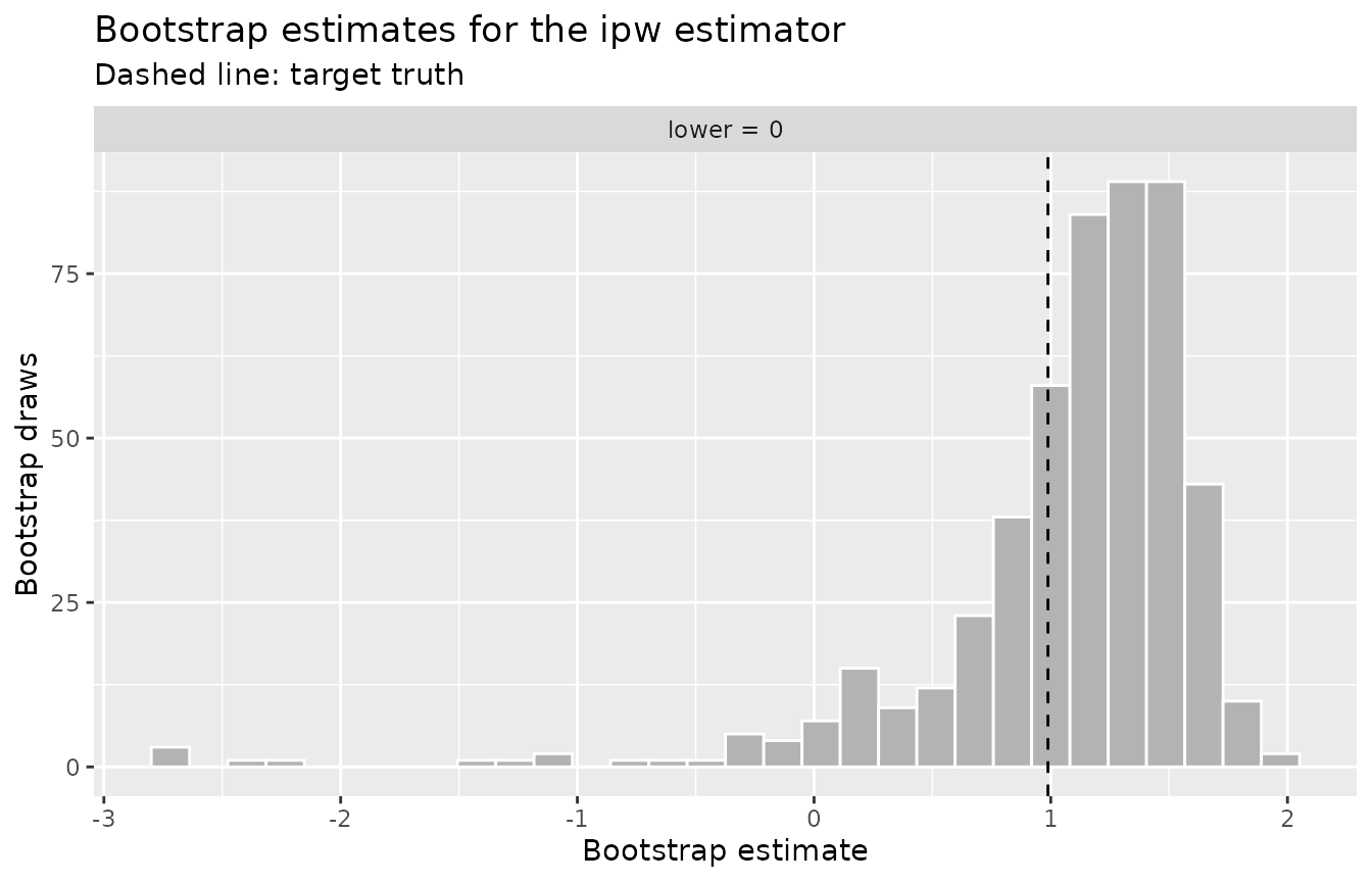
The three estimators respond differently, and running them on the same settings makes the contrast concrete. G-computation ignores the propensity altogether. The augmented, doubly robust estimator uses it and then corrects with the outcome model.
set.seed(1)
eta_gcomp <- check_eta_bias(
  eta_data,
  exposure,
  y,
  c(x1, x2),
  estimator = "gcomp",
  n_boot = 500
)

set.seed(1)
eta_aipw <- check_eta_bias(
  eta_data,
  exposure,
  y,
  c(x1, x2),
  estimator = "aipw",
  n_boot = 500
)

bind_rows(
  ipw = tidy(eta_ipw),
  gcomp = tidy(eta_gcomp),
  aipw = tidy(eta_aipw),
  .id = "estimator"
) |>
  select(estimator, bias, mc_se)
#> # A tibble: 3 × 3
#>   estimator     bias   mc_se
#>   <chr>        <dbl>   <dbl>
#> 1 ipw        0.0853  0.0274
#> 2 gcomp     -0.00223 0.00375
#> 3 aipw       0.0243  0.0161
G-computation sits within one Monte Carlo standard error of zero, which is what it should do: the target truth is itself a g-computation estimate, so the only distance between the two is bootstrap noise. The augmented estimator also sits within two standard errors of zero, its outcome-model correction absorbing most of the weighting bias, and it carries more variance than g-computation does. Inverse probability weighting is the estimator the violation reaches, which is why we diagnose it here.
The second use of the diagnostic evaluates truncation as a response
to the violation. Bounding the fitted propensity away from zero and one
before the estimator divides by it is a common reaction to extreme
weights, and it has a cost of its own. A vector of lower bounds passed
to truncation_grid becomes a set of truncation levels
c(lower, 1 - lower), and every level reuses one shared set
of bootstrap draws and model refits, so differences across the sweep
reflect the truncation bound alone. A lower bound of zero applies no
truncation, so the sweep can carry the untruncated run as its first
row.
set.seed(1)
sweep_result <- check_eta_bias(
  eta_data,
  exposure,
  y,
  c(x1, x2),
  estimator = "ipw",
  truncation_grid = c(0, 0.01, 0.05, 0.1),
  n_boot = 500
)
tidy(sweep_result)
#> # A tibble: 4 × 6
#>   term  truncation_lower truncation_upper   bias   mc_se boot_mean
#>   <chr>            <dbl>            <dbl>  <dbl>   <dbl>     <dbl>
#> 1 1 - 0             0                1    0.0853 0.0274       1.07
#> 2 1 - 0             0.01             0.99 0.232  0.0136       1.22
#> 3 1 - 0             0.05             0.95 0.592  0.00700      1.58
#> 4 1 - 0             0.1              0.9  0.901  0.00591      1.89
The first row and the rows below it say different things. The first
row is the untruncated level, and its bias belongs to the positivity
violation. Every row below it adds bias that the truncation rule
introduces, because the bound replaces the extreme fitted propensities
that carry the tail observations, and those are the observations the
weighting relies on to represent the tails of x1. By the
time the lower bound reaches 0.1, the bias the truncation rule has
introduced is an order of magnitude larger than the violation’s own. The
Monte Carlo standard error moves the other way, shrinking as the bound
tightens, because bounding the propensity stabilizes the weights. That
is the variance side of the tradeoff: truncation buys stability and pays
for it in bias.
The type = "sweep" plot shows ETA.Bias against the
truncation lower bound with a band of plus or minus two Monte Carlo
standard errors. The dashed line at zero marks the bias a
positivity-robust estimator would achieve.
autoplot(sweep_result, type = "sweep")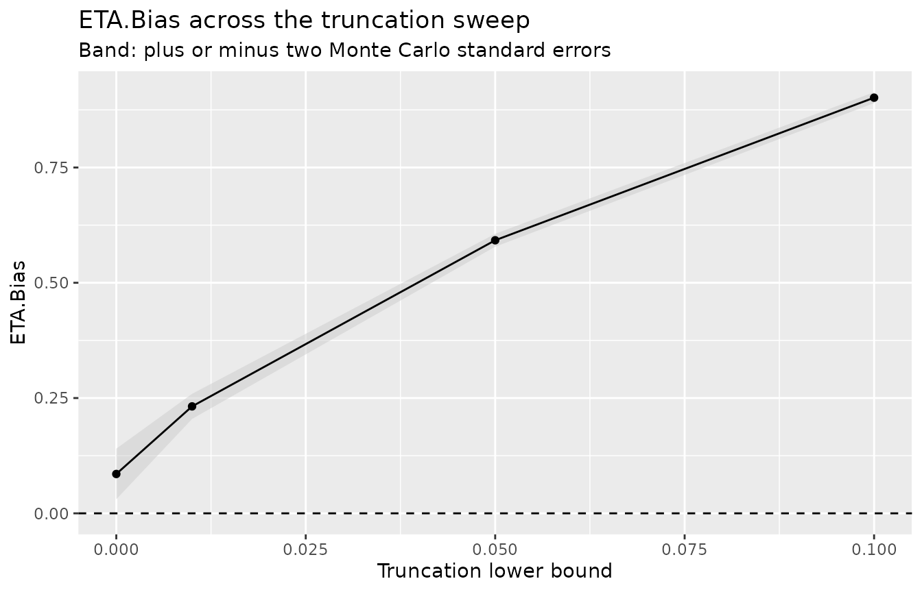
A categorical exposure, term by term
A binary exposure has one contrast to report. A categorical exposure
has one per non-reference level, and a positivity violation seldom
reaches them equally. The example below plants three doses whose top
level is nearly unreachable in the lower tail of x1, while
the middle level is well supported everywhere.
set.seed(2025)
n <- 400
x1 <- rnorm(n)
x2 <- rnorm(n)

# The odds of the top dose climb steeply in x1, so subjects in the lower tail
# of x1 almost never receive it.
odds <- cbind(1, exp(0.5 * x1), exp(-1.5 + 3 * x1))
probs <- odds / rowSums(odds)
dose <- factor(
  apply(probs, 1, function(p) sample(c("none", "low", "high"), 1, prob = p)),
  levels = c("none", "low", "high")
)

dose_data <- tibble(
  dose = dose,
  y = as.numeric(dose == "low") +
    2 * as.numeric(dose == "high") +
    2 * x1 + 0.5 * x2 + rnorm(n),
  x1 = x1,
  x2 = x2
)
count(dose_data, dose)
#> # A tibble: 3 × 2
#>   dose      n
#>   <fct> <int>
#> 1 none    155
#> 2 low     148
#> 3 high     97
Past two levels the treatment mechanism is a multinomial logit, fitted with the nnet package and refit on every bootstrap draw. The chunks in this section are gated on nnet being installed, so the vignette builds either way.
set.seed(1)
dose_ipw <- check_eta_bias(
  dose_data,
  dose,
  y,
  c(x1, x2),
  estimator = "ipw",
  n_boot = 200
)
#> ℹ Treating `.exposure` as categorical
tidy(dose_ipw)
#> # A tibble: 2 × 6
#>   term        truncation_lower truncation_upper    bias  mc_se boot_mean
#>   <chr>                  <dbl>            <dbl>   <dbl>  <dbl>     <dbl>
#> 1 low - none                 0               NA -0.0138 0.0321     0.828
#> 2 high - none                0               NA  0.306  0.0562     2.29
There is one row per non-reference level, and the two rows read
differently. The low - none contrast is within one Monte
Carlo standard error of zero: both levels are observed across the range
of x1, so weighting has support to work with. The
high - none contrast is biased upward by about five Monte
Carlo standard errors, which is the planted violation showing up in the
only estimand it touches. Reporting a single number for the whole
exposure would have averaged the two together and understated the
problem.
truncation_upper is missing on both rows because
truncation past two levels applies no upper bound. The paragraph on
truncation below unpacks that.
G-computation, which never divides by the fitted probabilities, sits within two Monte Carlo standard errors of zero on both terms.
set.seed(1)
dose_gcomp <- check_eta_bias(
  dose_data,
  dose,
  y,
  c(x1, x2),
  estimator = "gcomp",
  n_boot = 200
)

bind_rows(
  ipw = tidy(dose_ipw),
  gcomp = tidy(dose_gcomp),
  .id = "estimator"
) |>
  select(estimator, term, bias, mc_se)
#> # A tibble: 4 × 4
#>   estimator term           bias   mc_se
#>   <chr>     <chr>         <dbl>   <dbl>
#> 1 ipw       low - none  -0.0138 0.0321
#> 2 ipw       high - none  0.306  0.0562
#> 3 gcomp     low - none  -0.0157 0.00852
#> 4 gcomp     high - none -0.0153 0.0121
The type = "bootstrap" plot gives each term its own row
of facets, marked with the truth that term is aimed at. The two
distributions sit differently against their dashed lines, which is the
same reading the table gives.
autoplot(dose_ipw, type = "bootstrap")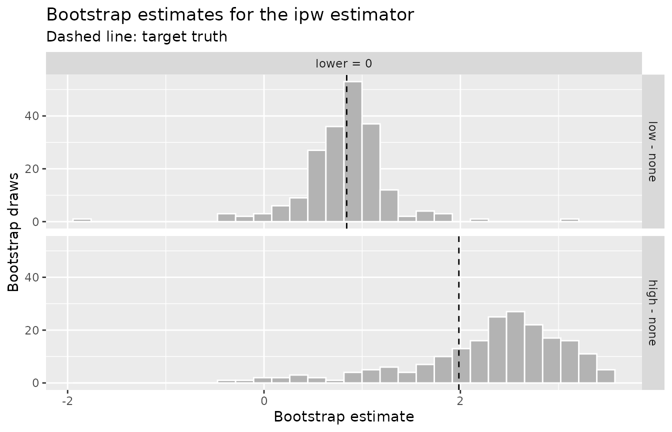
Both terms are contrasts against a reference level, none
here, which is the first factor level unless
reference_level names another. The reference is a choice of
parameterization rather than of estimand: the fitted mechanisms and the
bootstrap draws do not change with it, only which differences are
reported.
Truncation changes shape along with the estimand. With two levels the
fitted propensity has one free coordinate, so a grid entry
g bounds it into c(g, 1 - g). With more levels
each row of fitted probabilities is a point on a simplex, and a grid
entry raises every coordinate below g up to g
and renormalizes the row to sum to one, matching
propensity::ps_trunc(). Pinning every level away from zero
already bounds every weight denominator, so there is no upper bound to
apply, which is why truncation_upper is missing. A grid
entry has to sit below 1 / k for an exposure with
k levels, since k coordinates pinned at
1 / k already fill the simplex.
set.seed(1)
dose_sweep <- check_eta_bias(
  dose_data,
  dose,
  y,
  c(x1, x2),
  estimator = "ipw",
  truncation_grid = c(0, 0.02, 0.05, 0.1),
  n_boot = 200
)
tidy(dose_sweep)
#> # A tibble: 8 × 6
#>   term        truncation_lower truncation_upper     bias  mc_se boot_mean
#>   <chr>                  <dbl>            <dbl>    <dbl>  <dbl>     <dbl>
#> 1 low - none              0                  NA -0.0138  0.0321     0.828
#> 2 low - none              0.02               NA -0.00664 0.0239     0.836
#> 3 low - none              0.05               NA  0.0305  0.0185     0.873
#> 4 low - none              0.1                NA  0.0777  0.0144     0.920
#> 5 high - none             0                  NA  0.306   0.0562     2.29
#> 6 high - none             0.02               NA  0.617   0.0310     2.60
#> 7 high - none             0.05               NA  0.949   0.0229     2.93
#> 8 high - none             0.1                NA  1.32    0.0198     3.31
The rows walk the sweep once per term. The high - none
bias more than quadruples across the grid while the
low - none bias stays under a tenth, so the truncation rule
charges almost all of its bias to the contrast that was already the
weakest. The Monte Carlo standard error falls on both terms, the
variance side of the same tradeoff the binary sweep showed.
autoplot(dose_sweep, type = "sweep")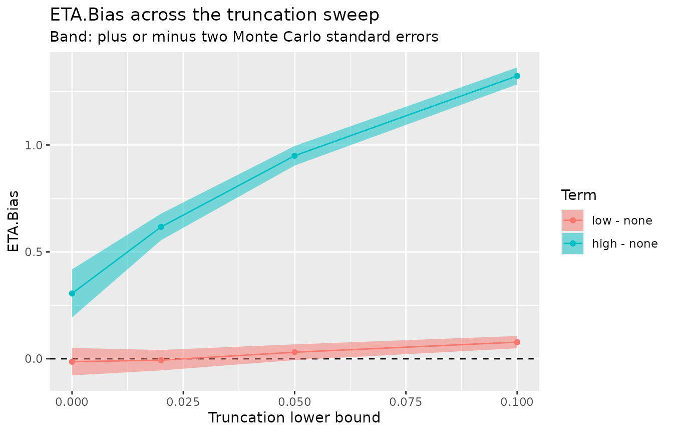
A continuous exposure and its working model
A continuous exposure has no levels to contrast, so the estimand is
the coefficient set of a marginal structural model.
msm_formula sets that working model, and the default is
linear in the exposure. The weights differ too: inverse probability
weighting for a continuous exposure divides by a density rather than by
a probability, weighting each observation by the stabilized density
ratio, the marginal density of the exposure over its conditional density
given the covariates.
That ratio is what a sharp treatment mechanism makes explosive. The
example plants one: x1 explains nine tenths of the variance
in the dose, so the conditional density is far tighter than the marginal
and the few observations whose dose is unusual for their covariates
carry enormous weight.
set.seed(2025)
n <- 400
x1 <- rnorm(n)
x2 <- rnorm(n)

infusion <- tibble(
  x1 = x1,
  x2 = x2,
  dose = 1.5 * x1 + 0.5 * rnorm(n)
) |>
  mutate(y = dose + 2 * x1 + 0.5 * x2 + rnorm(n))
set.seed(1)
infusion_ipw <- check_eta_bias(
  infusion,
  dose,
  y,
  c(x1, x2),
  estimator = "ipw",
  n_boot = 200
)
#> ℹ Treating `.exposure` as continuous
infusion_ipw
#>
#> ── ETA bias ────────────────────────────────────────────────────────────────────
#> Exposure: "dose" (continuous)
#> Observations: 400
#> Estimator: ipw
#> Bootstrap draws: 200
#> Truth: 1.093
#> ETA.Bias: 0.848 (MC SE 0.017)
The term is named dose, the one non-intercept
coefficient of the default working model, and the truth is that
coefficient under the observed fit: the counterfactual mean outcome is
evaluated over the deciles of the observed dose and projected onto the
working model by least squares. The bias is more than three quarters of
the truth, which is what a mechanism this sharp does to a density-ratio
weight. G-computation, reading the same fitted outcome model, sits on
zero.
set.seed(1)
infusion_gcomp <- check_eta_bias(
  infusion,
  dose,
  y,
  c(x1, x2),
  estimator = "gcomp",
  n_boot = 200
)
tidy(infusion_gcomp)
#> # A tibble: 1 × 6
#>   term  truncation_lower truncation_upper     bias   mc_se boot_mean
#>   <chr>            <dbl>            <dbl>    <dbl>   <dbl>     <dbl>
#> 1 dose                NA              Inf -0.00343 0.00753      1.09
Because the working model defines the estimand rather than
approximating one, two analyses of these data that set different
msm_formula values are aimed at different targets and will
report different biases. That is a property of the estimand and not an
inconsistency: the number reported is the bias of estimating the working
model the analysis actually uses, so it is worth reading beside the
formula that produced it.
Truncation is the third thing that changes with the type. There is no
probability to bound, so a grid entry g caps the stabilized
weight at its 1 - g quantile, read once from the observed
fit and held fixed across the bootstrap draws. The augmented estimator
is unavailable here, and truncation and
reference_level are errors rather than silent no-ops.
set.seed(1)
infusion_sweep <- check_eta_bias(
  infusion,
  dose,
  y,
  c(x1, x2),
  estimator = "ipw",
  truncation_grid = c(0, 0.01, 0.05, 0.1),
  n_boot = 200
)
tidy(infusion_sweep)
#> # A tibble: 4 × 6
#>   term  truncation_lower truncation_upper  bias   mc_se boot_mean
#>   <chr>            <dbl>            <dbl> <dbl>   <dbl>     <dbl>
#> 1 dose                NA          Inf     0.848 0.0168       1.94
#> 2 dose                NA            6.89  0.942 0.00799      2.03
#> 3 dose                NA            1.47  1.03  0.00481      2.12
#> 4 dose                NA            0.813 1.07  0.00414      2.16
truncation_lower is missing at every level, since there
is no lower cap to place on a density ratio, and
truncation_upper holds the cap itself: infinite where no
truncation was applied, then the weight at each requested quantile. The
caps say how concentrated the ratio is, falling from about seven at the
0.99 quantile of the weights to under one at the 0.9 quantile. The bias
says that capping does not rescue the estimator. It grows slightly as
the cap tightens while the Monte Carlo standard error falls by a factor
of four, so truncation buys stability around an answer that is wrong by
most of the target either way.
autoplot(infusion_sweep, type = "sweep")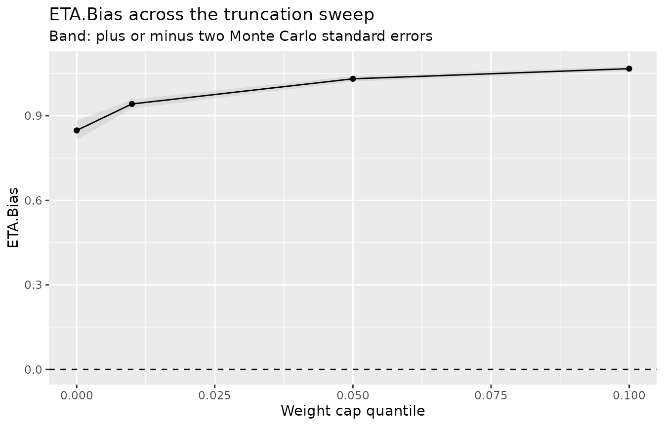
ETA.Bias captures the positivity, truncation, and sparsity component of bias and excludes model-misspecification bias by construction. It reports a diagnostic for a fitted mechanism and does not correct the estimate.
Extrapolation as the g-computation view of positivity
G-computation predicts the outcome under each exposure value for
every unit and averages the contrast. It never divides by the
propensity, so it does not produce the extreme weights that a positivity
violation creates for inverse probability weighting. The violation does
not disappear, though. It changes form. Where one exposure group has no
member near a unit’s covariate profile, g-computation must predict that
unit’s outcome under the missing exposure by extrapolating the model
beyond the data it was trained on. Under g-computation the positivity
problem becomes an extrapolation problem, and
check_extrapolation() measures it directly.
check_extrapolation() implements the extrapolation
diagnostics of King and Zeng (2006). For every observation it measures
how well the opposite exposure group covers that unit’s position in
covariate space, using Gower distances that handle numeric and
categorical covariates together. We pass all three covariates, including
the factor region.
extrapolation <- check_extrapolation(
  pos_violations,
  exposure,
  c(x1, x2, region)
)
extrapolation
#>
#> ── Extrapolation ───────────────────────────────────────────────────────────────
#> Exposure: "exposure" (binary)
#> Observations: 1000
#> Geometric variability: 0.144
#> Nearby radius (1 x gv): 0.144
#> Mean fraction nearby: 0.284
#> Nearest opposite within one geometric variability: 999 of 1000
#> In opposite-group hull: 784 of 1000
The Gower distance between two rows is the mean over covariates of a
per-covariate distance: for a numeric covariate, the absolute difference
divided by the pooled sample range; for a factor, one when the
categories differ and zero when they agree. Distances lie in
[0, 1]. The geometric variability is one half the mean of
the full distance matrix and sets the reference radius: an observation
counts an opposite-group unit as nearby when their Gower distance is
within one geometric variability, controlled by the nearby
multiplier.
Three per-unit statistics are reported: gower_min, the
distance to the nearest opposite-group unit; gower_mean,
the mean distance to the opposite group; and frac_nearby,
the fraction of the opposite group within the reference radius.
tidy(extrapolation)
#> # A tibble: 1,000 × 7
#>      .id exposure frac_nearby gower_min gower_mean in_hull low_support
#>    <int>    <int>       <dbl>     <dbl>      <dbl> <lgl>   <lgl>
#>  1     1        1       0.325   0.0223       0.291 TRUE    FALSE
#>  2     2        1       0.380   0.00566      0.276 TRUE    FALSE
#>  3     3        0       0.386   0.00837      0.255 TRUE    FALSE
#>  4     4        0       0.426   0.00384      0.247 TRUE    FALSE
#>  5     5        1       0.297   0.0113       0.302 TRUE    FALSE
#>  6     6        1       0.220   0.0281       0.325 TRUE    FALSE
#>  7     7        1       0.284   0.0197       0.304 TRUE    FALSE
#>  8     8        0       0.321   0.00920      0.302 TRUE    FALSE
#>  9     9        0       0.223   0.0323       0.330 FALSE   FALSE
#> 10    10        0       0.269   0.0286       0.322 TRUE    FALSE
#> # ℹ 990 more rows
The units with the lowest frac_nearby sit in the
covariate tails and in the structural subgroup, the same regions PoRT
reports. The type = "distribution" plot shows the
distribution of frac_nearby within each exposure group.
Most units carry a third to a half of the opposite group nearby, and the
thin left tail is the handful with almost none, whose g-computation
prediction under the missing exposure rests on extrapolation.
autoplot(extrapolation, type = "distribution")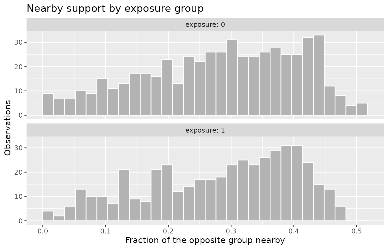
The convex-hull test is the sharper statement of the same idea. It
asks whether each observation lies inside the convex hull of the
opposite group, solved as a linear-programming feasibility problem on
the numeric covariates. A unit outside the opposite group’s hull cannot
be written as a weighted average of opposite-group units, so any
g-computation prediction for it under the missing exposure is
extrapolation by construction. The test runs automatically when there
are at most ten numeric covariates and the lpSolve package is installed;
lpSolve is a suggested dependency, so install it to enable the hull
test. summary() aggregates the results by exposure group,
reporting the fraction of each group inside the opposite group’s
hull.
summary(extrapolation)
#> # A tibble: 2 × 5
#>   exposure     n mean_gower_min prop_supported prop_in_hull
#>      <int> <int>          <dbl>          <dbl>        <dbl>
#> 1        0   542         0.0269          0.998        0.686
#> 2        1   458         0.0191          1            0.900
The type = "hull" plot shows how many units of each
group fall inside the opposite group’s hull. The units outside it are
the ones that require extrapolation, and they include the structural
subgroup that is never exposed.
autoplot(extrapolation, type = "hull")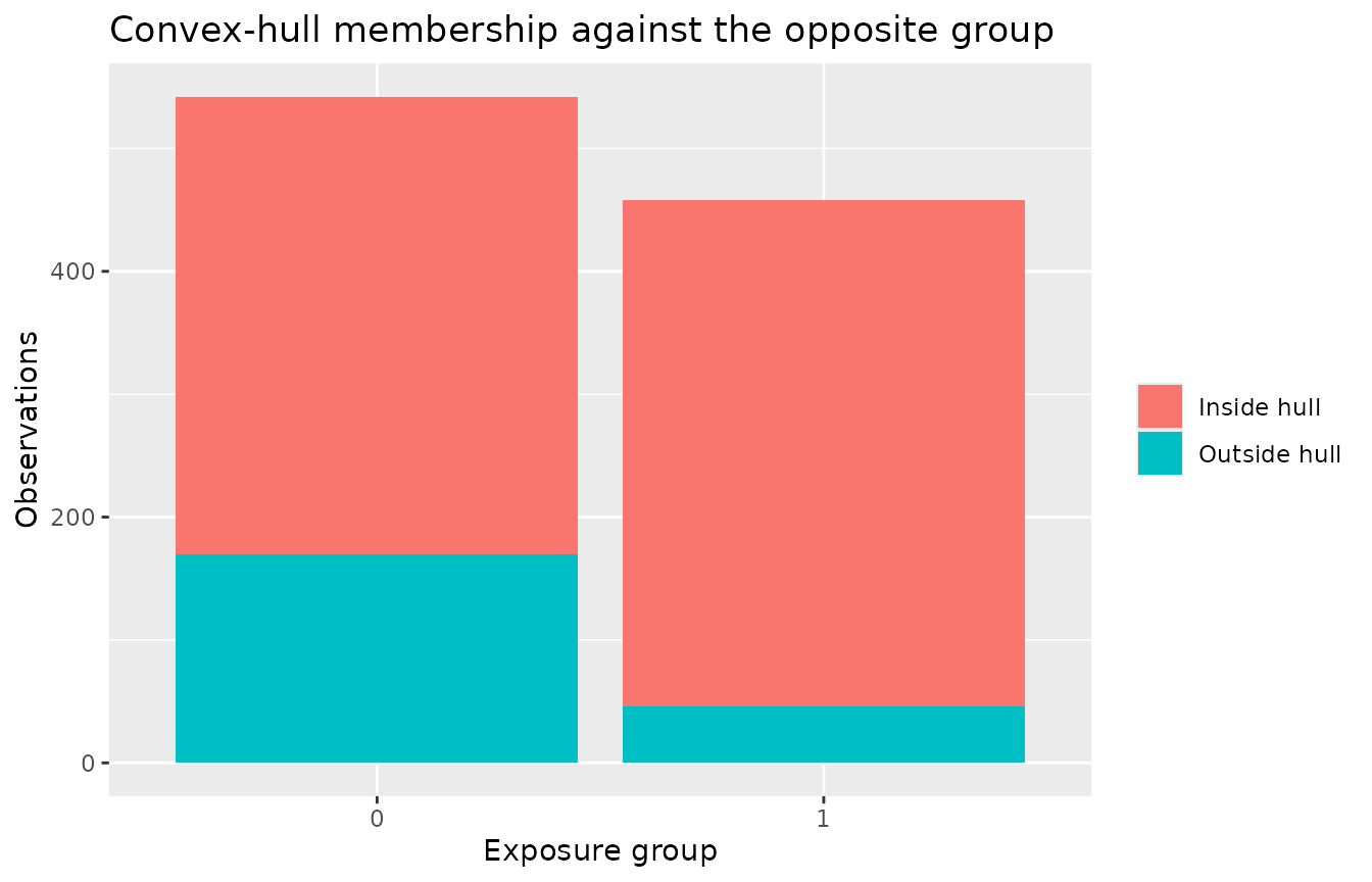
Read together, the two diagnostics describe the same positivity violation from the estimator’s side. ETA.Bias puts a number on what the violation costs the inverse-probability-weighting estimator, and on what truncating the weights would cost on top of that, and the extrapolation check shows the g-computation estimator leaning on model predictions for the units in the tails and the structural subgroup.
Where to go next
The getting-started vignette, Getting started with
positively, covers check_positivity() end to end and
the diagnostics that answer whether positivity holds. The vignette
Density ratios and modified treatment policies covers
check_density_ratios(), the diagnostic for stochastic and
modified treatment policies, with hand-built ratios and with a fitted
longitudinal model.
References
King G, Zeng L (2006). The Dangers of Extreme Counterfactuals. Political Analysis, 14(2):131-159. doi:10.1093/pan/mpj004
Petersen ML, Porter KE, Gruber S, Wang Y, van der Laan MJ (2012). Diagnosing and responding to violations in the positivity assumption. Statistical Methods in Medical Research, 21(1):31-54. doi:10.1177/0962280210386207