Positivity for continuous exposures

For a binary exposure, a positivity problem has a familiar shape: the fitted propensity approaches zero or one, and there are two tails to inspect. A continuous exposure has no single propensity to threshold. Positivity becomes a question about support: for each candidate dose and each stratum of the covariates, is there observed data near that dose? A violation is a region of the joint exposure-covariate space that holds little or no data, and that region does not reduce to two tails. It can sit in the middle of the exposure range, it can depend on the covariates, and it can be invisible in the marginal distribution of the exposure. The three continuous-exposure diagnostics in positively measure support in three different ways, and each is informative about a different geometry of violation.

Setup

library(positively)
library(dplyr)

positively includes pos_violations_long, a simulated wide-format longitudinal dataset with one row per subject over three time points. Each exposure column is continuous, taking hundreds of distinct values.

pos_violations_long
#> # A tibble: 500 × 7
#>       id      l0     a1      l1    a2    l2     a3
#>    <int>   <dbl>  <dbl>   <dbl> <dbl> <dbl>  <dbl>
#>  1     1  0.621  -0.672  0.202   5.32 7.49   6.77 
#>  2     2  0.0356  2.00  -0.0732  5.71 4.79   7.89 
#>  3     3  0.773   1.30   0.688   4.35 4.19   2.96 
#>  4     4  1.27    2.23   0.808   5.40 4.06   4.64 
#>  5     5  0.371   1.75   1.01    1.31 1.33   1.36 
#>  6     6 -0.163  -0.920 -1.64    1.78 0.507 -0.197
#>  7     7  0.397  -0.936 -1.73    5.74 6.09   8.04 
#>  8     8 -0.0800 -1.14  -0.804   5.25 5.56   5.70 
#>  9     9 -0.345  -0.976 -1.03    5.77 5.43   2.37 
#> 10    10  0.702   0.532  0.287   4.55 6.15   6.43 
#> # ℹ 490 more rows

The planted violation is documented in ?pos_violations_long and lives in the time-2 exposure a2. That exposure is drawn on [0, 2] or [4, 6], so it never falls in the open interval (2, 4). The time-1 and time-3 exposures place values throughout that interval, so the gap is specific to a2 rather than a feature of the exposure process as a whole.

range(pos_violations_long$a2)
#> [1] 0.006241528 5.997213255
any(pos_violations_long$a2 > 2 & pos_violations_long$a2 < 4)
#> [1] FALSE

The sections below run each diagnostic on a2 with the covariates l0 and l1. The gap is a mid-support hole in the marginal distribution of a2, so it is a useful case for showing which diagnostic detects which kind of violation.

Effective data points: support at chosen exposure values

check_edp() computes the effective-data-points diagnostic of Ring and Schomaker (2026). For each observation moved to a candidate intervention value, it sums a product kernel over the sample to measure how much observed data surrounds that intervened-on point. The result runs from zero, meaning no observed support, up to the sample size.

For a continuous exposure the default candidate values are the deciles of the observed exposure, which follow the observed mass and here all fall outside the gap. To probe the suspected hole, supply candidate values that span the range, including one inside the gap.

edp <- check_edp(pos_violations_long, a2, c(l0, l1), values = c(1, 3, 5))
#> ℹ Treating `.exposure` as continuous
edp
#> 
#> ── Effective data points ───────────────────────────────────────────────────────
#> Exposure: "a2" (continuous)
#> Observations: 500
#> Variant: data
#> Intervention values: 3
#> edp range: 0.896 to 95.254

The message reports that the exposure was detected as continuous. Detection runs once per call, but only a diagnostic that supports more than one exposure type announces what it settled on: check_edp() computes a different quantity for each type it accepts, so which one it read is worth saying. A diagnostic that supports a single type has nothing to report, so check_hat_values() and check_hdr() below stay silent, as does any call that declares the type. Detection is a default and not an override: the section on declaring the exposure type shows how to set the type yourself when the heuristic reads a continuous exposure as something else.

Effective data points are a relative measure, meaningful when compared across candidate values for a fixed covariate set rather than against a universal threshold. The candidate value 3 sits in the gap. Summarizing by candidate value shows its effective data points are far below those at the supported values 1 and 5.

tidy(edp) |>
  group_by(value) |>
  summarize(edp = round(mean(edp), 1))
#> # A tibble: 3 × 2
#>   value   edp
#>   <dbl> <dbl>
#> 1     1  59.6
#> 2     3  21.4
#> 3     5  62.2

The autoplot() histogram, faceted by candidate value, shows the same result as a distribution. The mass for the gap value 3 is concentrated at low effective data points, while the supported values carry a broad distribution of well supported observations.

autoplot(edp, type = "histogram")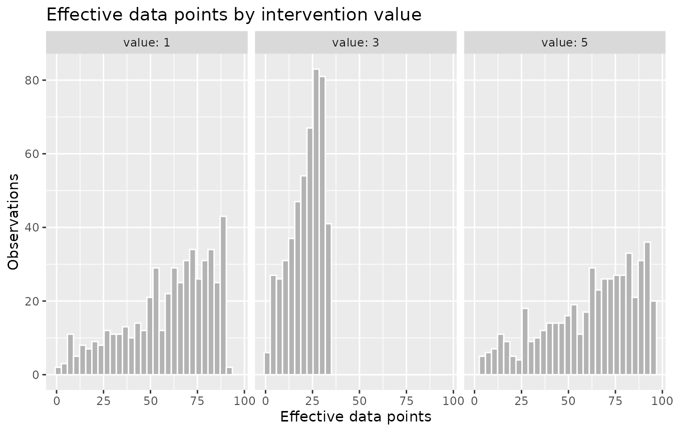

Effective data points detect the a2 gap directly, because the kernel measures local support in the joint exposure-covariate space without assuming a form for the conditional density.

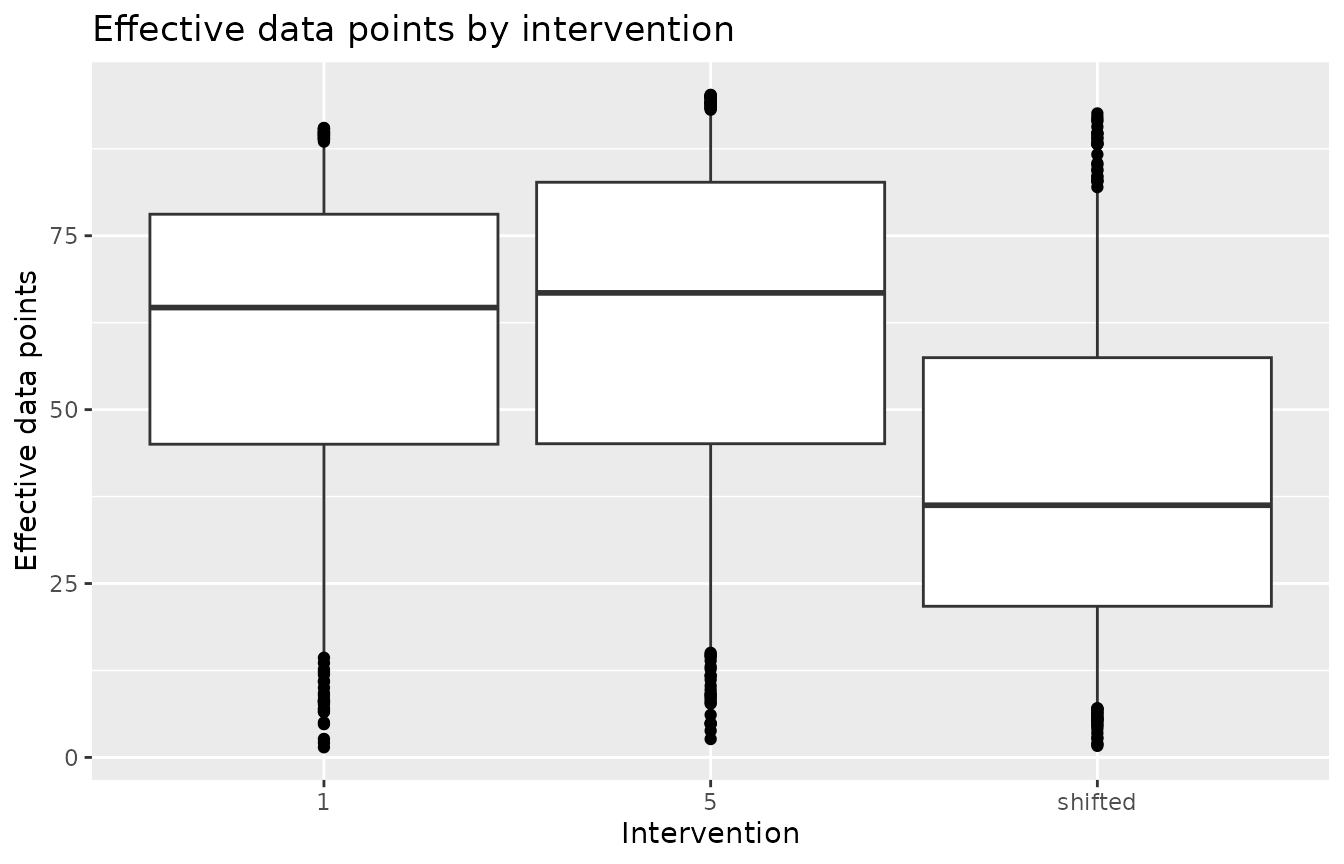
Hat values: leverage-based extrapolation risk

check_hat_values() computes the hat-value diagnostic of Moodie and Schulz (2025). It fits the linear design matrix formed from the exposure and the covariates, then for each exposure percentile and each observed covariate row it measures the leverage that the resulting candidate point would exert on the model. A candidate is flagged as high leverage when its hat value exceeds threshold * p / n. The summary statistic is the proportion of high-leverage candidates, calibrated against a null in which the exposure is drawn independently of the covariates.

The null distribution is drawn by resampling, so we set a seed in the chunk. We use null_reps = 100 to keep the vignette fast. This is a toy setting; in practice keep at least the default of 500 replicates so that the null quantile is stable.

set.seed(1)
hat_values <- check_hat_values(
  pos_violations_long,
  a2,
  c(l0, l1),
  null_reps = 100
)
hat_values
#> 
#> ── Hat values ──────────────────────────────────────────────────────────────────
#> Exposure: "a2" (continuous)
#> Observations: 500
#> Null: permutation (100 reps), cutoff 2p/n
#> phi-hat: 0.065
#> Null 0.95 quantile: 0.065
#> Exceeds null: FALSE
#> High-leverage candidates: 613 of 9500

The observed summary statistic does not exceed the null quantile, so the leverage profile is not distinguishable from one in which the exposure and covariates are independent. Two properties of the diagnostic explain the result. First, the candidate exposure values are percentiles of the observed exposure, which fall on the two supported modes and never enter the gap. Second, a2 does not depend strongly on l0 or l1, so no exposure-covariate combination is far from the observed design in the leverage sense.

autoplot(hat_values, type = "null")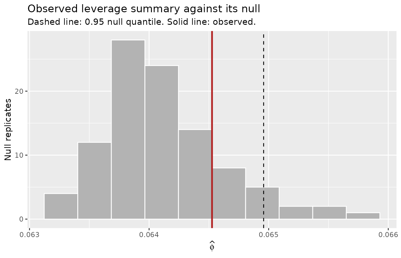

Hat values identify extrapolation risk that arises when specific exposure values combine with covariate values in a way that is far from the observed design. That risk is present when the exposure is covariate-driven, and it is evaluated at plausible exposure percentiles rather than at holes in the exposure’s own support. The a2 gap is a marginal mid-support hole, so it falls outside what hat values measure.

Highest density region non-overlap

check_hdr() computes the highest-density-region non-overlap ratio of Bao and Schomaker (2025). For a common target exposure value, it reports the fraction of covariate profiles whose highest-density region excludes that value, that is, the share of the population for which the target dose is not supported. The ratio is zero when the target is supported everywhere and one when it is supported nowhere.

hdr <- check_hdr(pos_violations_long, a2, c(l0, l1))
hdr
#> 
#> ── HDR non-overlap ─────────────────────────────────────────────────────────────
#> Exposure: "a2" (continuous)
#> Observations: 500
#> HDR mass: 0.95
#> Density estimator: normal
#> Non-overlap over 100 targets: 0 to 0

The non-overlap ratio is zero at every target, including targets inside the gap. The default estimator, hdr_density_normal(), fits lm(a2 ~ l0 + l1) and treats the conditional density as Gaussian around the fitted mean. The a2 gap is a hole between two modes of the conditional density, and the fitted normal fills that hole and reports the target as supported. As documented in ?check_hdr, the default estimator detects mean-shift support gaps, where a stratum’s supported dose moves away from a target, and does not detect multimodal gaps. A flexible conditional-density estimator supplied through new_hdr_density() is needed to detect a multimodal hole.

To show the ratio when it is informative, consider a mean-shift example in which the exposure depends strongly on a covariate.

set.seed(2)
n <- 500
l <- rnorm(n)
dose <- rnorm(n, mean = 2 * l, sd = 0.4)
shift <- data.frame(dose = dose, l = l)

hdr_shift <- check_hdr(shift, dose, l)
hdr_shift
#> 
#> ── HDR non-overlap ─────────────────────────────────────────────────────────────
#> Exposure: "dose" (continuous)
#> Observations: 500
#> HDR mass: 0.95
#> Density estimator: normal
#> Non-overlap over 100 targets: 0.706 to 0.996

Here each covariate stratum supports a narrow band of doses around its own mean, so no single common dose is supported across the whole population. The non-overlap ratio has a nonzero floor even at the central target, and it rises toward one for extreme targets. The autoplot() curve shows the ratio against the target value.

autoplot(hdr_shift)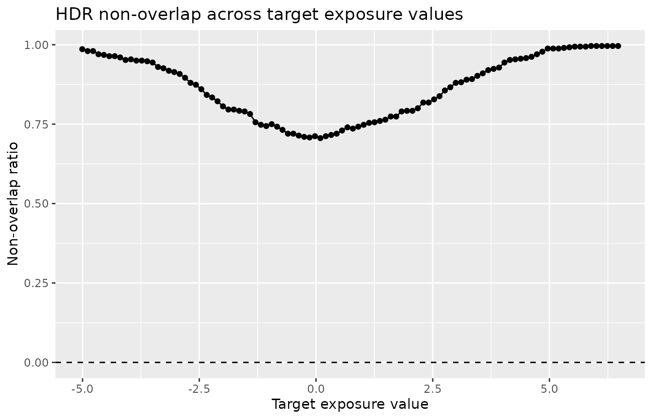

The non-overlap ratio measures support for a common target dose across covariate strata. It is a population-level quantity: a nonzero floor means that setting the whole population to one dose is infeasible, not that the density model fits poorly.

When each diagnostic is informative

The three diagnostics measure support in different ways, so they detect different geometries of violation.

• Effective data points measure local support in the joint exposure-covariate space at candidate exposure values you choose. They detect sparse support at those values, including a mid-support hole in the exposure’s own distribution, as with the a2 gap.
• Hat values measure leverage-based extrapolation risk for exposure percentiles combined with observed covariate rows. They are informative when the exposure is covariate-driven and extreme dose-covariate combinations sit far from the observed design. They do not target holes in the exposure’s marginal support.
• Highest density region non-overlap measures whether a common target dose falls within the highest-density region of each covariate stratum. With the default normal estimator it detects mean-shift gaps, where a stratum’s supported dose moves away from the target, and requires a flexible density estimator to detect multimodal holes.

Running all three and reading them together shows both the location of a violation and the kind of support it lacks.

Declaring the exposure type

Every diagnostic infers the exposure type from the data unless you declare it. Exactly two distinct values is read as binary; otherwise a numeric exposure is read as categorical when fewer than 20 percent of its values are distinct, which is a sensible default and the wrong answer for a coarsely measured dose. Consider a drug dose recorded at eight milligram levels across 150 subjects, with higher doses given to subjects with higher l.

set.seed(3)
n <- 150
l <- rnorm(n)
dose <- round(pmin(pmax(35 + 15 * l + rnorm(n, sd = 5), 0), 70) / 10) * 10
coarse <- data.frame(dose = dose, l = l)

sort(unique(coarse$dose))
#> [1]  0 10 20 30 40 50 60 70

The dose is continuous in every sense that matters to these diagnostics, but eight distinct values over 150 observations fall well under the cutoff, so it is detected as categorical.

check_edp(coarse, dose, l, values = c(10, 40, 70))
#> ℹ Treating `.exposure` as categorical
#> 
#> ── Effective data points ───────────────────────────────────────────────────────
#> Exposure: "dose" (categorical)
#> Observations: 150
#> Variant: data
#> Intervention values: 3
#> edp range: 0 to 38.891

check_edp() accepts a categorical exposure, so it runs regardless, treating each dose level as a category. check_hat_values() and check_hdr() do not accept one, so under detection alone neither would run here at all. Setting exposure_type settles the question. A declared type is authoritative: detection is not consulted at all, and the declaration is refused only when its math cannot run on the column as given, which for "continuous" means a column that is not numeric and for "binary" a column without exactly two distinct values.

check_hdr(coarse, dose, l, values = c(10, 40, 70), exposure_type = "continuous")
#> 
#> ── HDR non-overlap ─────────────────────────────────────────────────────────────
#> Exposure: "dose" (continuous)
#> Observations: 150
#> HDR mass: 0.95
#> Density estimator: normal
#> Non-overlap over 3 targets: 0.42 to 0.967

The non-overlap ratio is lowest at 40, near the center of the observed doses, and highest at the two extremes, which few covariate profiles support.

check_positivity() takes the same argument and forwards the resolved type to every diagnostic it composes, so one declaration covers the whole set.

set.seed(4)
check_positivity(coarse, dose, l, exposure_type = "continuous")
#> 
#> ── Positivity check ────────────────────────────────────────────────────────────
#> Exposure: "dose" (continuous); 150 observations; covariate l
#> 
#> ── port ────────────────────────────────────────────────────────────────────────
#> 20 subgroups reported, 6 with low support
#> Rule: prevalence outside [0.05, 0.95] among subgroups of at least 5% of the
#> sample
#> 
#> ── hat_values ──────────────────────────────────────────────────────────────────
#> phi-hat 0.51 exceeds the 0.95 permutation-null quantile of 0.044
#> 1453 of 2850 unit-value pairs above the 2p/n cutoff (500 reps)
#> 
#> ── edp ─────────────────────────────────────────────────────────────────────────
#> Data variant over 5 intervention values; edp 0.109 to 49.94
#> 
#> ── hdr ─────────────────────────────────────────────────────────────────────────
#> 95% HDR, normal density; non-overlap 0.413 to 0.967 over 100 targets
#> 
#> ℹ `sniff_violations()` for what was found, `$port` to extract a diagnostic,
#> `summary()` for every statistic.

Each diagnostic offers only the types it supports, so "binary" is not among check_hdr()’s choices and declaring it there fails on the argument rather than on the column. check_positivity() takes all three types, so it is where the structural rule does the refusing: eight distinct doses are not two.

check_positivity(coarse, dose, l, exposure_type = "binary")
#> Error in `check_positivity()`:
#> ! `check_positivity()` needs exactly two distinct values in `.exposure`
#>   for a binary exposure.
#> ✖ `.exposure` has 8 distinct values.

Time-varying exposures

check_hdr_seq() applies the non-overlap ratio to a time-varying continuous exposure, one time point at a time, fitting the conditional density of each exposure on the history that enters its conditioning set. It accepts the same wide-format data used above, with an ordered selection of exposure columns and a per-time-point list of covariates. The Identifying violations: PoRT and sPoRT vignette covers the sequential diagnostics in full, including conditioning-set construction and the longitudinal support structure of pos_violations_long.

Where to go next

The Getting started with positively vignette introduces check_positivity() and reads each diagnostic’s output and plot on a binary example. For a continuous exposure, check_positivity() runs effective data points, positivity regression trees with the exposure categorized, hat values, and highest density region non-overlap together, with the defaults used above.

References

Bao Y, Schomaker M (2025). Feasible Dose-Response Curves for Continuous Treatments Under Positivity Violations.

Moodie EEM, Schulz J (2025). A Simple Diagnostic for the Positivity Assumption for Continuous Exposures. Statistics in Medicine, 44:e70194.

Ring C, Schomaker M (2026). A Diagnostic to Find and Help Combat Stochastic Positivity Issues, with a Focus on Continuous Treatments.