A ggplot2 geom for plotting ROC curves with optional weighting. Emphasizes the balance interpretation where AUC around 0.5 indicates good balance.
Usage
geom_roc(
  mapping = NULL,
  data = NULL,
  stat = "roc",
  position = "identity",
  na.rm = TRUE,
  show.legend = NA,
  inherit.aes = TRUE,
  linewidth = 0.5,
  .focal_level = NULL,
  ...
)
Arguments
- mapping
Set of aesthetic mappings. Must include
estimate(propensity scores/predictions) andexposure(treatment/outcome variable). If specified, inherits from the plot.- data
Data frame to use. If not specified, inherits from the plot.
- stat
Statistical transformation to use. Default is "roc".
- position
Position adjustment. Default is "identity".
- na.rm
If
FALSE, the default, missing values are removed with a warning. IfTRUE, missing values are silently removed.- show.legend
Logical. Should this layer be included in the legends?
NA, the default, includes if any aesthetics are mapped.- inherit.aes
If
FALSE, overrides the default aesthetics, rather than combining with them.- linewidth
Width of the ROC curve line. Default is 0.5.
- .focal_level
The level of the
exposureaesthetic to treat as the event. Must be a level the data actually takes; a declared factor level that no observation takes is not accepted. IfNULL(default), the last observed level is used, which is the maximum value for numeric exposures.- ...
Other arguments passed on to layer().
Details
A curve compares two exposure levels, so each curve is drawn from the rows
that share an aesthetic signature, with the exposure level excluded from that
signature. Mapping group explicitly makes each group a curve of its own,
which keeps long data holding several weighting schemes from being pooled
into a single curve. A group that holds only one observed exposure level is
dropped with a warning, and the remaining curves are still drawn.
See also
check_model_auc() for computing AUC values, stat_roc() for the underlying stat
Other ggplot2 functions:
geom_calibration(),
geom_ecdf(),
geom_mirror_density(),
geom_mirror_histogram(),
geom_qq2()
Examples
# Basic usage
library(ggplot2)
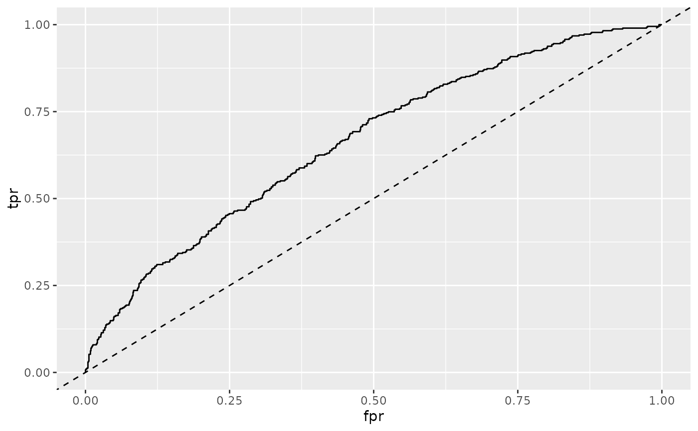
ggplot(nhefs_weights, aes(estimate = .fitted, exposure = qsmk)) +
geom_roc() +
geom_abline(intercept = 0, slope = 1, linetype = "dashed")
 # With grouping by weight
long_data <- tidyr::pivot_longer(
nhefs_weights,
cols = c(w_ate, w_att),
names_to = "weight_type",
values_to = "weight"
)
#> Warning: Converting psw to numeric: incompatible estimands 'ate' and 'att'
#> ℹ Metadata cannot be preserved when combining incompatible objects
#> ℹ Use identical objects or explicitly cast to numeric to avoid this warning
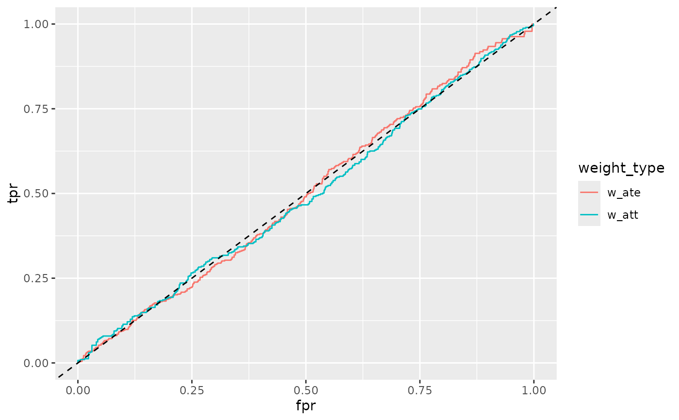
ggplot(long_data, aes(estimate = .fitted, exposure = qsmk, weight = weight)) +
geom_roc(aes(color = weight_type)) +
geom_abline(intercept = 0, slope = 1, linetype = "dashed")
# With grouping by weight
long_data <- tidyr::pivot_longer(
nhefs_weights,
cols = c(w_ate, w_att),
names_to = "weight_type",
values_to = "weight"
)
#> Warning: Converting psw to numeric: incompatible estimands 'ate' and 'att'
#> ℹ Metadata cannot be preserved when combining incompatible objects
#> ℹ Use identical objects or explicitly cast to numeric to avoid this warning
ggplot(long_data, aes(estimate = .fitted, exposure = qsmk, weight = weight)) +
geom_roc(aes(color = weight_type)) +
geom_abline(intercept = 0, slope = 1, linetype = "dashed")