Plot an ETA.Bias diagnostic

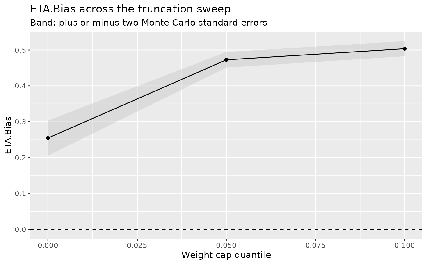
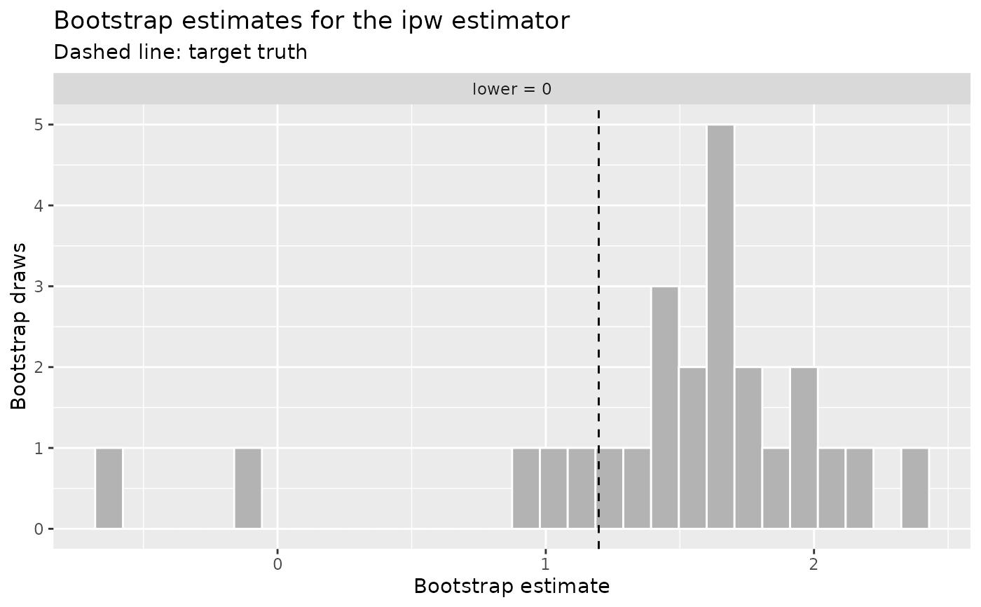
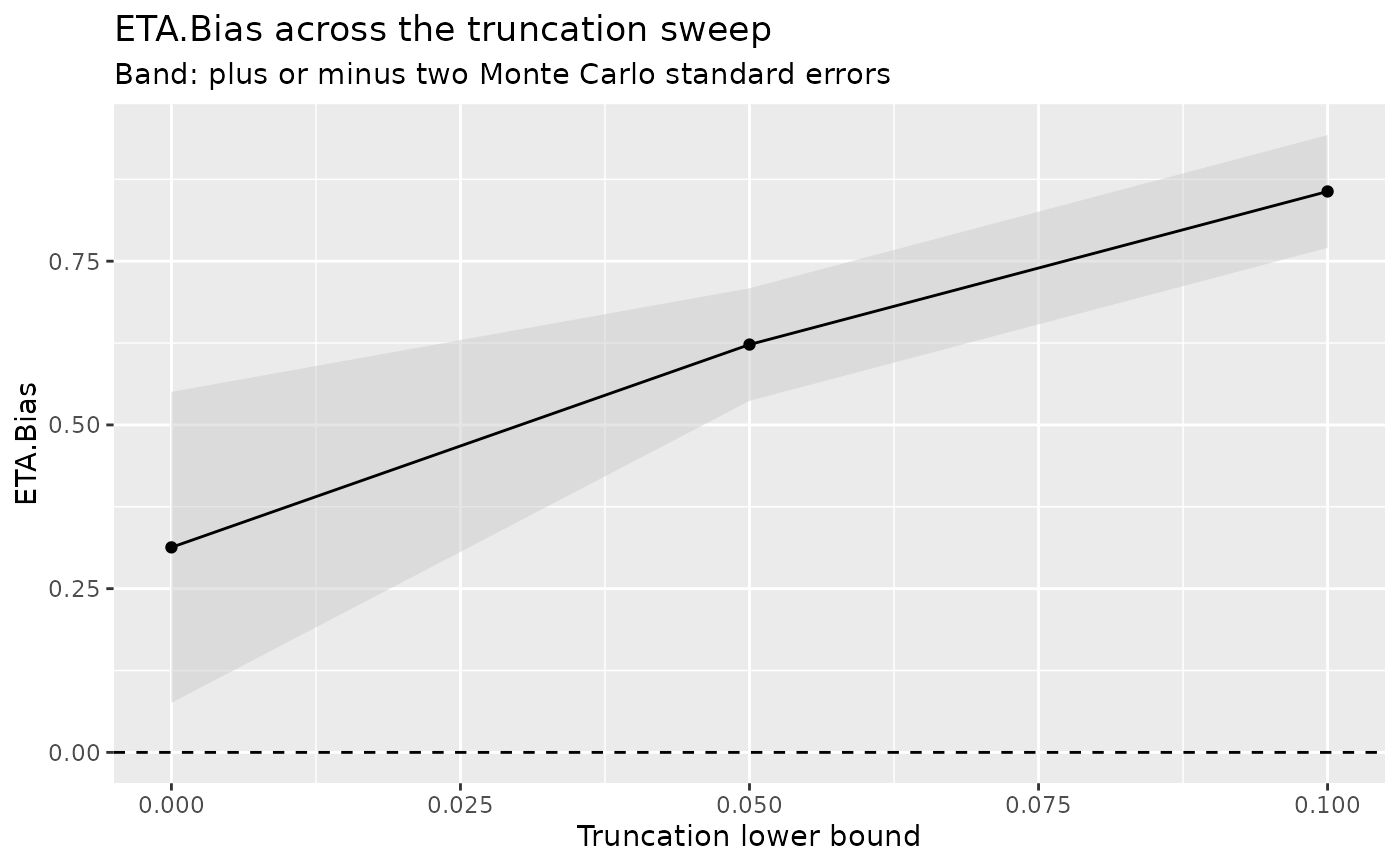
Draws one of two views of a check_eta_bias() result. type = "bootstrap" shows the distribution of bootstrap estimates as a histogram, one facet per estimand term and truncation level, each facet marking the truth its term is aimed at. type = "sweep" shows ETA.Bias with a two-Monte-Carlo-standard-error band across the truncation sweep, the bias-variance tradeoff of weight truncation, with one line per estimand term.

Arguments

object

An eta_bias_result from check_eta_bias().

type

One of "bootstrap" or "sweep".

...

Not used.

Value

A ggplot2::ggplot object.

Details

An estimand of one term, read at one truncation level, draws a single facet. A discrete exposure truncates a fitted probability, so its sweep is drawn against the truncation lower bound. A continuous exposure caps a stabilized weight instead and reports no probability bound at any level, so its sweep is drawn against the quantile levels those caps were read at.

Examples

set.seed(1)
n <- 300
x1 <- rnorm(n)
x2 <- rnorm(n)
a <- rbinom(n, 1, plogis(2 * (x1 + x2)))
y <- a + x1 + x2 + rnorm(n)
df <- data.frame(a = a, y = y, x1 = x1, x2 = x2)
# n_boot is small here to keep the example fast.
result <- check_eta_bias(df, a, y, c(x1, x2), n_boot = 25)
#> ℹ Treating `.exposure` as binary
autoplot(result, type = "bootstrap")


swept <- check_eta_bias(
  df,
  a,
  y,
  c(x1, x2),
  truncation_grid = c(0, 0.05, 0.1),
  n_boot = 25
)
#> ℹ Treating `.exposure` as binary
autoplot(swept, type = "sweep")


# A continuous exposure caps its weights at a quantile, so the sweep reads
# the quantile levels rather than a probability bound.
df$a <- x1 + x2 + rnorm(n)
df$y <- df$a + x1 + x2 + rnorm(n)
continuous <- check_eta_bias(
  df,
  a,
  y,
  c(x1, x2),
  truncation_grid = c(0, 0.05, 0.1),
  n_boot = 25
)
#> ℹ Treating `.exposure` as continuous
autoplot(continuous, type = "sweep")