Get started with balancing

Balancing weights target covariate balance directly. Instead of fitting a model for the probability of exposure and deriving weights from it, a balancing method poses covariate balance as a convex optimization problem and solves for the weights that achieve it. This vignette walks through the core workflow for a binary exposure: fitting weights with balance(), reading the balance they achieve, checking that balance more broadly with halfmoon, and estimating a causal effect.

# halfmoon provides the balance-assessment tools used throughout this
# vignette.
library(halfmoon)
library(balancing)

A confounded example

We simulate a study with two confounders, age and score, a binary exposure, and a continuous outcome. Both confounders drive the exposure and the outcome, so a naive comparison of exposed and unexposed units is biased.

n <- 800
age <- rnorm(n)
score <- rnorm(n)
exposure <- rbinom(n, 1, plogis(0.5 * age - 0.6 * score))
outcome <- 1 + 0.8 * exposure + 0.7 * age - 0.5 * score + rnorm(n)

study <- data.frame(exposure, age, score, outcome)

Before weighting, the exposed and unexposed groups differ on both confounders. halfmoon’s check_balance() summarizes that imbalance; the observed rows are the unweighted sample, where the standardized mean differences on age and score run to about half a standard deviation in opposite directions. The same call appears again later with the weights attached.

check_balance(study, c(age, score), exposure)
#> # A tibble: 7 × 5
#>   variable group_level method   metric estimate
#>   <chr>    <chr>       <chr>    <chr>     <dbl>
#> 1 age      0           observed ks        0.229
#> 2 age      0           observed smd       0.544
#> 3 age      0           observed vr        1.14 
#> 4 score    0           observed ks        0.214
#> 5 score    0           observed smd      -0.510
#> 6 score    0           observed vr        0.868
#> 7 NA       NA          observed energy    0.234

Fitting balancing weights

balance() takes the data frame, the exposure and covariate columns selected with tidyselect, a method specification, and an estimand. We start with entropy balancing for the average treatment effect on the treated (ATT), which reweights the unexposed group to match the covariate means of the exposed group.

fit <- balance(
  study,
  exposure,
  c(age, score),
  method = bw_entropy(),
  estimand = "att"
)

fit
#> 
#> ── Entropy balancing ───────────────────────────────────────────────────────────
#> Exposure: "exposure" (binary)
#> Estimand: "att" (focal level "1")
#> Observations: 800
#> Solver: converged in 4 iterations
#> Constraints: 2 terms (tolerance 0)
#> Largest imbalance: 0.0000 (standardized mean difference)

The print method summarizes the fit. It reports the method and the exposure type detected from the data, the estimand and its focal level, the number of observations, whether the solver converged, and the largest imbalance the weights leave on the constraint terms. Here the largest standardized mean difference is effectively zero: entropy balancing achieves exact mean balance by construction.

Checking balance with halfmoon

The balance table reports balance on the terms the weights were asked to balance. To assess balance more broadly, including statistics beyond the mean and variables the weights did not target, extract the weights with weights() and pass them to the halfmoon package.

study$w <- weights(fit)

Passing the weights to the same check_balance() call compares the weighting scheme against the unweighted sample across a set of covariates.

balance_check <- check_balance(
  study,
  c(age, score),
  exposure,
  .weights = w
)
balance_check
#> # A tibble: 14 × 5
#>    variable group_level method   metric  estimate
#>    <chr>    <chr>       <chr>    <chr>      <dbl>
#>  1 age      0           observed ks      2.29e- 1
#>  2 age      0           w        ks      6.15e- 2
#>  3 age      0           observed smd     5.44e- 1
#>  4 age      0           w        smd     2.64e-15
#>  5 age      0           observed vr      1.14e+ 0
#>  6 age      0           w        vr      1.09e+ 0
#>  7 score    0           observed ks      2.14e- 1
#>  8 score    0           w        ks      6.31e- 2
#>  9 score    0           observed smd    -5.10e- 1
#> 10 score    0           w        smd    -6.90e-15
#> 11 score    0           observed vr      8.68e- 1
#> 12 score    0           w        vr      1.10e+ 0
#> 13 NA       NA          observed energy  2.34e- 1
#> 14 NA       NA          w        energy  7.49e- 3

plot_balance() renders the same comparison as a love plot.

plot_balance(balance_check)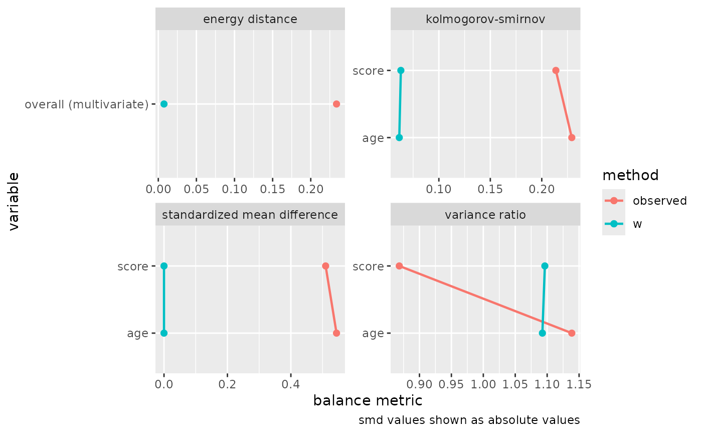

halfmoon owns the general balance-assessment workflow, so its love plots, mirrored histograms, and balance summaries are the place to look when you want a fuller picture than the constraint terms provide. It also reports the effective sample size, the amount of each group that survives weighting, through check_ess().

Estimating a causal effect

The weights are a bw vector. weights() returns the balancing weights already multiplied by any sampling weights, so its result goes straight into a weighted outcome model; there is no need to compose the sampling weights yourself. Manual composition is only called for when you have weights from a separate source that the fit does not carry. With a marginal outcome model, the exposure coefficient is the weighted effect estimate.

outcome_mod <- lm(outcome ~ exposure, data = study, weights = w)
coef(outcome_mod)[["exposure"]]
#> [1] 0.7705934

The estimate recovers the simulated effect of 0.8, which the unweighted comparison would have missed.

Standard errors with `ipw()`

A weighted outcome model’s usual standard errors treat the weights as fixed, but the weights were themselves estimated. For the estimating-equation methods (entropy balancing, inverse probability tilting, and the just-identified covariate balancing propensity score) with a binary or categorical exposure, and for entropy balancing with a continuous one, ipw() returns effect estimates with standard errors that account for the estimation of the weights.

binary_outcome <- rbinom(n, 1, plogis(-0.3 + 0.6 * exposure + 0.4 * age))
study$event <- binary_outcome

ate_fit <- balance(
  study,
  exposure,
  c(age, score),
  method = bw_entropy(),
  estimand = "ate"
)
study$w_ate <- weights(ate_fit)

event_mod <- glm(
  event ~ exposure,
  data = study,
  family = quasibinomial(),
  weights = w_ate
)

ipw(ate_fit, event_mod)
#> Inverse Probability Weight Estimator
#> Estimand: ATE 
#> Effects: marginal (population-averaged) 
#> 
#> Weight Estimator:
#>   Call: balance(.data = study, .exposure = exposure, .covariates = c(age, 
#>     score), method = bw_entropy(), estimand = "ate") 
#> 
#> Outcome Model:
#>   Call: glm(formula = event ~ exposure, family = quasibinomial(), data = study, 
#>     weights = w_ate) 
#> 
#> Marginal estimates:
#>         estimate  std.err      z ci.lower ci.upper conf.level   p.value    
#> rd      0.134288 0.036908 3.6385  0.06195  0.20663       0.95 0.0002743 ***
#> log(rr) 0.263052 0.073661 3.5711  0.11868  0.40742       0.95 0.0003554 ***
#> log(or) 0.540819 0.150477 3.5940  0.24589  0.83575       0.95 0.0003256 ***
#> ---
#> Signif. codes:  0 '***' 0.001 '**' 0.01 '*' 0.05 '.' 0.1 ' ' 1

The vignette("inference") article explains why these standard errors differ from the naive ones and how to obtain valid intervals for the methods that do not carry estimating equations.

Where to go next