Silverman (1985): Generalized Additive Model • deli

Note

This article is translated from the Silverman (1985): Generalized Additive Model example in the documentation of delicatessen, deli’s Python counterpart.

library(deli)
library(ggplot2)

theme_set(theme_minimal())

The following is a brief illustrative example of how generalized additive models (GAMs) can be implemented using M-estimation. For demonstration, we use data on motorcycle impacts from Silverman (1985).

Loading Data

The motorcycle data contains measurements of head acceleration (in g) over time (in ms) during simulated motorcycle impacts. The relationship between time and acceleration is clearly non-linear.

# Load the motorcycle data from the MASS package
d <- MASS::mcycle

# Format data for deli
X <- cbind(1, d$times)
y <- d$accel

# Create prediction grid
p_times <- seq(min(d$times), max(d$times), length.out = 200)
Xp <- cbind(1, p_times)

Linear Regression

As easily seen in the scatterplot, the relationship between time and acceleration is non-linear. We can show this further by fitting a regression model with a linear relationship between the variables.

# Define estimating equation for linear regression
estr <- m_estimate(
  stacked_equations = function(theta) {
    ee_regression(theta, X = X, y = y, model = "linear")
  },
  init = c(0, 0)
)

# Predicted values and confidence intervals
pred_y <- regression_predictions(Xp, coef(estr), vcov(estr))

# Plot
fit_curve <- data.frame(
  times = p_times,
  accel = pred_y$predicted,
  lower = pred_y$lower,
  upper = pred_y$upper
)

ggplot(fit_curve, aes(x = times, y = accel)) +
  geom_point(data = d, size = 1) +
  geom_ribbon(aes(ymin = lower, ymax = upper), fill = "orange", alpha = 0.3) +
  geom_line(color = "orange", linewidth = 1) +
  labs(x = "Time (ms)", y = "Acceleration (g)")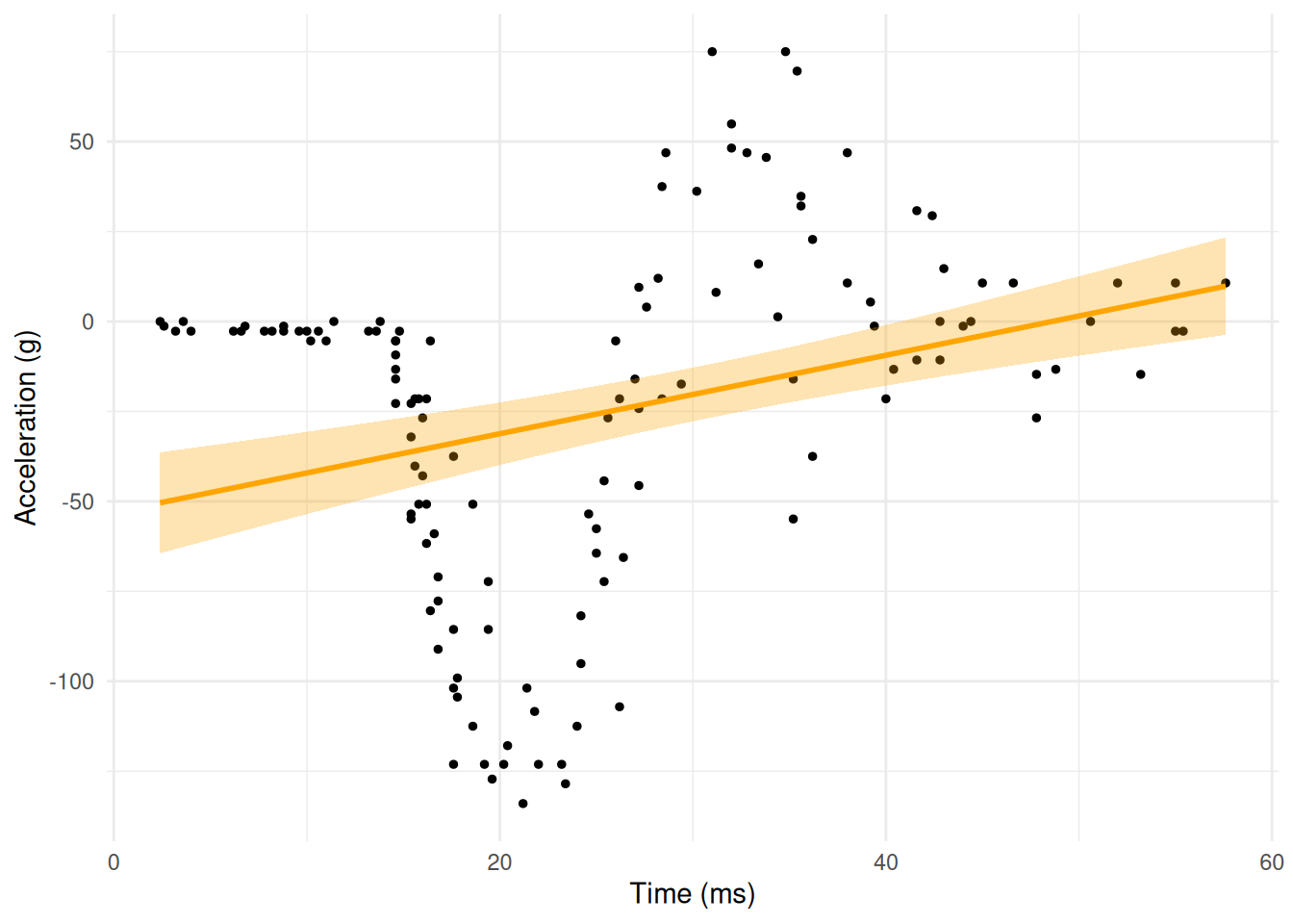

As we can clearly see, a linear relationship is very different from the observed data.

Implementing a GAM

GAMs are implemented through the use of L_2-penalized splines. The user needs to provide the knot locations (or number of knots). Other optional arguments include the power of the splines, whether to restrict, and the strength of the penalty. Stronger penalties move the model closer to the fit of a linear model.

For the intercept term, we do not want any splines. For times, we specify 11 knots and a penalty of 2000, which together with the intercept and linear term give 12 parameters. This penalty prevents the GAM from being too “wiggly”.

# Define knot locations at percentiles of times
knot_locs <- as.numeric(quantile(d$times, probs = seq(0.025, 0.975, length.out = 11)))

# Specifications for the additive design matrix
specs <- list(
  NULL,                                                    # No spline for intercept
  list(knots = knot_locs, penalty = 2000, power = 3)       # Spline for times
)

# Define estimating equation for additive regression
estr <- m_estimate(
  stacked_equations = function(theta) {
    ee_additive_regression(
      theta, X = X, y = y,
      model = "linear",
      specifications = specs
    )
  },
  init = rep(0, 12)
)
#> Warning: ! The estimating equations are rank deficient at the returned values, so the
#>   parameters are not identified.
#> ℹ At least one direction in the parameter space leaves the mean estimating
#>   equations unchanged, so they have no unique root and every point along that
#>   direction solves them as well as the values returned here.
#> ℹ Results may be unreliable. Check the equations for a redundant parameter and
#>   the design for linearly dependent columns.

# Build the additive design matrix for predictions
Xpa <- additive_design_matrix(Xp, specifications = specs)

# Generate predicted values
pred_y <- regression_predictions(Xpa, coef(estr), vcov(estr))

# Plot
fit_curve <- data.frame(
  times = p_times,
  accel = pred_y$predicted,
  lower = pred_y$lower,
  upper = pred_y$upper
)

ggplot(fit_curve, aes(x = times, y = accel)) +
  geom_point(data = d, size = 1) +
  geom_ribbon(aes(ymin = lower, ymax = upper), fill = "orange", alpha = 0.3) +
  geom_line(color = "orange", linewidth = 1) +
  labs(x = "Time (ms)", y = "Acceleration (g)")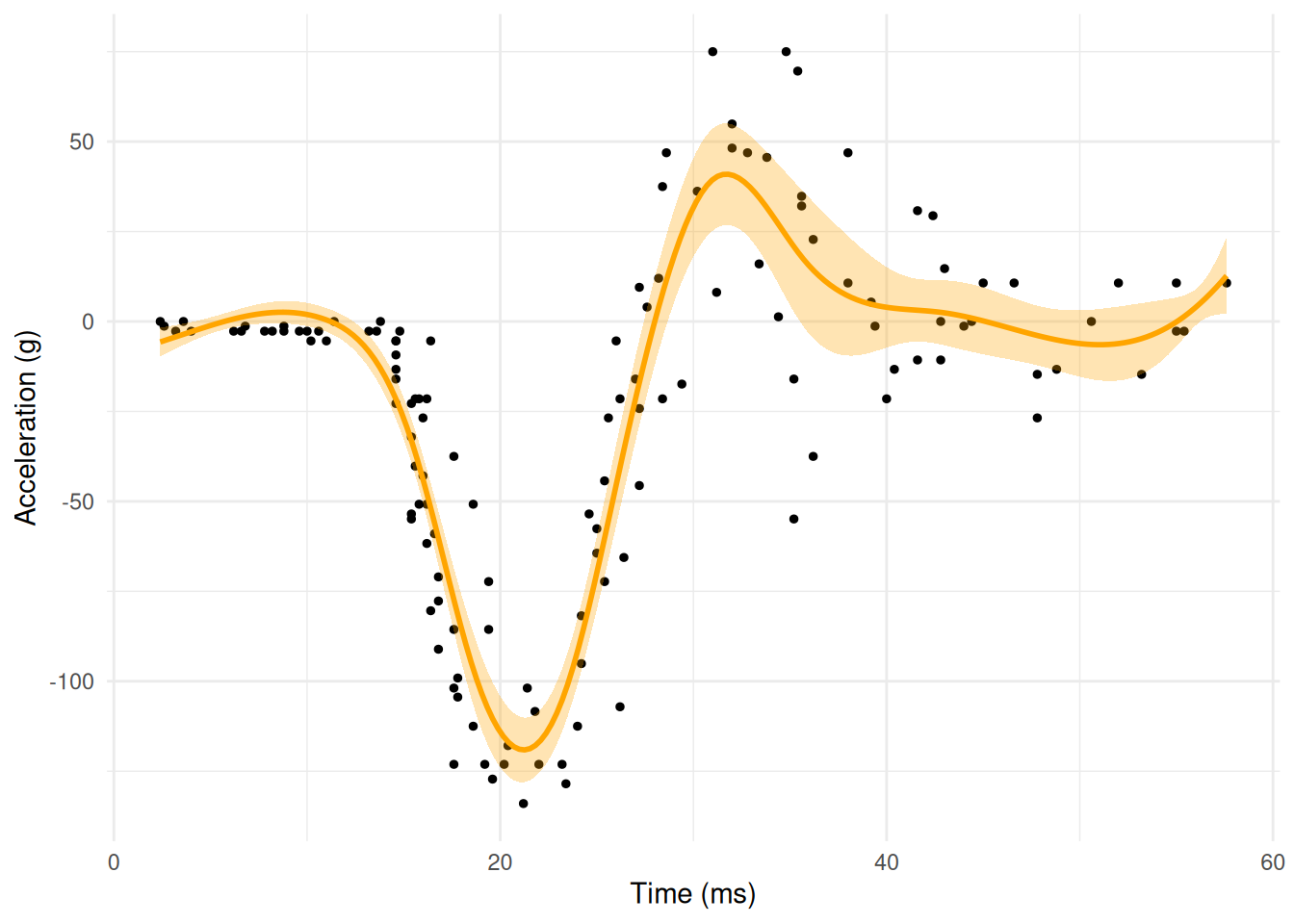

The GAM does a much better job of following the shape of the scatterplot.

Impact of the Penalty

To show how the penalty impacts the wiggliness of the GAM, let’s increase the penalty by a large amount. As this penalty is only applied to the spline terms, we would expect to see the regression line become smoother.

Strong Penalty (1,000,000)

# Increase the penalty
specs_strong <- list(
  NULL,
  list(knots = knot_locs, penalty = 1000000, power = 3)
)

estr <- m_estimate(
  stacked_equations = function(theta) {
    ee_additive_regression(
      theta, X = X, y = y,
      model = "linear",
      specifications = specs_strong
    )
  },
  init = rep(0, 12)
)

# Build additive design matrix and predict
Xpa <- additive_design_matrix(Xp, specifications = specs_strong)
pred_y <- regression_predictions(Xpa, coef(estr), vcov(estr))

# Plot
fit_curve <- data.frame(
  times = p_times,
  accel = pred_y$predicted,
  lower = pred_y$lower,
  upper = pred_y$upper
)

ggplot(fit_curve, aes(x = times, y = accel)) +
  geom_point(data = d, size = 1) +
  geom_ribbon(aes(ymin = lower, ymax = upper), fill = "orange", alpha = 0.3) +
  geom_line(color = "orange", linewidth = 1) +
  labs(x = "Time (ms)", y = "Acceleration (g)")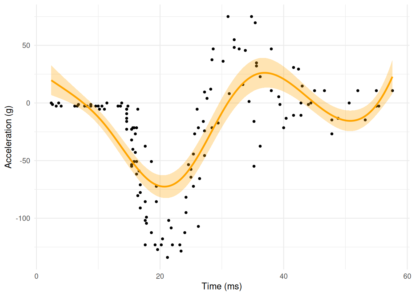

The estimated function from the GAM is smoother than the previous GAM. Let’s crank up the penalty even further.

Very Strong Penalty (100,000,000,000)

# Very large penalty
specs_vstrong <- list(
  NULL,
  list(knots = knot_locs, penalty = 1e11, power = 3)
)

estr <- m_estimate(
  stacked_equations = function(theta) {
    ee_additive_regression(
      theta, X = X, y = y,
      model = "linear",
      specifications = specs_vstrong
    )
  },
  init = rep(0, 12)
)

# Build additive design matrix and predict
Xpa <- additive_design_matrix(Xp, specifications = specs_vstrong)
pred_y <- regression_predictions(Xpa, coef(estr), vcov(estr))

# Plot
fit_curve <- data.frame(
  times = p_times,
  accel = pred_y$predicted,
  lower = pred_y$lower,
  upper = pred_y$upper
)

ggplot(fit_curve, aes(x = times, y = accel)) +
  geom_point(data = d, size = 1) +
  geom_ribbon(aes(ymin = lower, ymax = upper), fill = "orange", alpha = 0.3) +
  geom_line(color = "orange", linewidth = 1) +
  labs(x = "Time (ms)", y = "Acceleration (g)")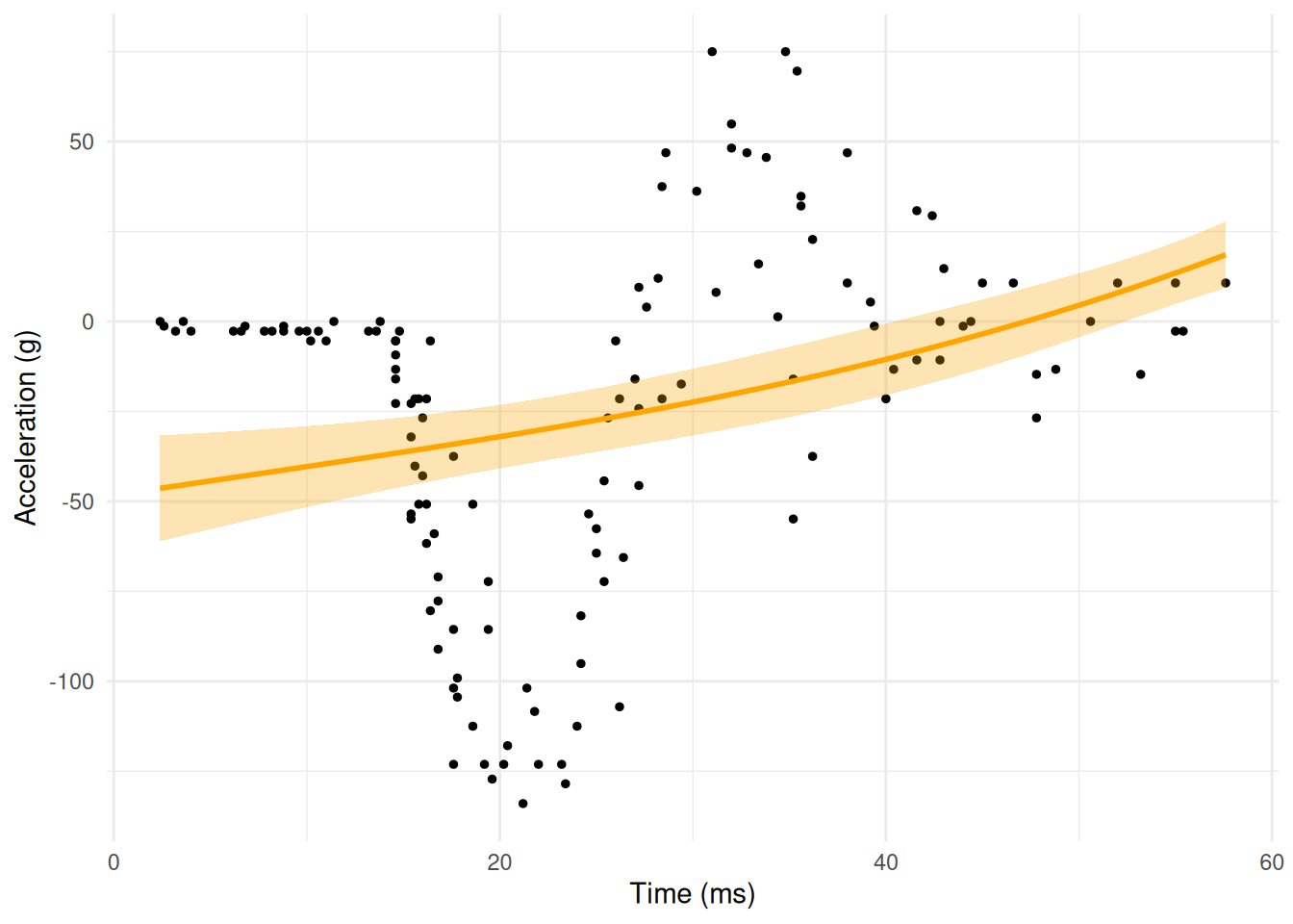

Here, the GAM is very similar to the linear regression we started with. This demonstrates the general relationship: as the penalty goes to infinity, the GAM will coincide with the linear model.

To summarize, we want a penalty that prevents overfitting to the data but does not prevent the GAM from approximating the data. This selection of penalization is commonly done via cross-validation. However, use of cross-validation invalidates standard variance estimation approaches (including with the sandwich variance estimator). Therefore, we recommend sacrificing the optimal penalty parameter (as determined by cross-validation) in favor of simpler variance estimation.

GAMs are a flexible method that place fewer constraints on the functional forms of relationships via splines. These splines do not require us to know the true underlying functional form. Instead, the higher-order splines (with well-chosen knots) can serve as close approximations.

References

Silverman BW. (1985). Some aspects of the spline smoothing approach to non-parametric regression curve fitting. Journal of the Royal Statistical Society: Series B (Methodological), 47(1), 1-21.