Collett (2015): Survival Analysis

Note

This article is translated from the Collett (2015): Survival Analysis example in the documentation of delicatessen, deli’s Python counterpart.

library(deli)
library(ggplot2)

theme_set(theme_minimal())

The following presents some survival analysis methods framed as M-estimators. The described example and methods are detailed further in the book by Collett. In survival analysis, we are commonly interested in estimating the survival or risk at a particular time. However, some observations are censored (most commonly right censored, which is exclusively considered hereafter). Therefore, our data is composed of the observation time (T^*) and an event indicator (\Delta). The observation time is usually framed as the minimum of the time-to-event (T) and time-to-censor (C). Here, we assume that each person has both times, but we only see T^* = \min(T,C). The event indicator tells us which of these two options occurred (\Delta = 1 if it was the event). Therefore, survival analysis methods consider how to efficiently learn functions of the time-to-event variable with this partial missingness. See Collett for a more detailed review of survival analysis and its methods.

Data

Here, data on the survival times of 45 women with breast cancer in Middlesex Hospital July 1987 (Table 1.2) is used. Information was collected on whether tumors were positively or negatively stained with HPA. This will be the only covariate included in the analysis.

# Load the breast cancer data from the deli package
d <- breast_cancer
d$C <- 1

# Time points for drawing survival functions
times_to_predict <- seq(0.5, 230, length.out = 100)

Here, time (or times in R) is the observation time, status (or delta in R) is the event indicator, and stain is whether the tumor was HPA stained positive or negative. This data set can also be loaded via breast_cancer in the R deli package.

Chapter 5: Parametric Proportional Hazards Models

To begin, we will simply model the survival times using parametric models without covariates.

Exponential

The exponential model is a one parameter model that assumes the hazard is constant. It is the simplest of the survival models. This model is parameterized as h(t) = \lambda The following code can be used to fit the exponential model.

# Define the estimating equation for the exponential survival model
psi <- function(theta) {
  ee_survival_model(theta = theta,
                    time = d$times,
                    event = d$delta,
                    distribution = "exponential")
}

# Fit the M-estimator
estr <- m_estimate(stacked_equations = psi, init = c(0.01))

# Display the results
results <- data.frame(
  Est = coef(estr),
  SE = sqrt(diag(vcov(estr))),
  LCL = confint(estr)[, 1],
  UCL = confint(estr)[, 2],
  row.names = c("Lambda")
)
round(results, 3)
#>          Est    SE   LCL   UCL
#> Lambda 0.006 0.001 0.003 0.009

So the estimated hazard at each time is simply 0.006.

Another more informative way to view the results from this model is to plot the estimated survival function. The following code generates the confidence intervals for the survival function at designated times using the Delta Method.

# Compute survival predictions with confidence intervals
surv <- survival_predictions(
  times = times_to_predict,
  theta = coef(estr),
  covariance = vcov(estr),
  distribution = "exponential"
)

# Plot the survival function
ggplot(surv, aes(x = time, y = predicted)) +
  geom_ribbon(aes(ymin = lower, ymax = upper), fill = "black", alpha = 0.3) +
  geom_line() +
  coord_cartesian(xlim = c(0, 235), ylim = c(0, 1)) +
  labs(x = "Time (months)", y = "Survival", title = "Exponential")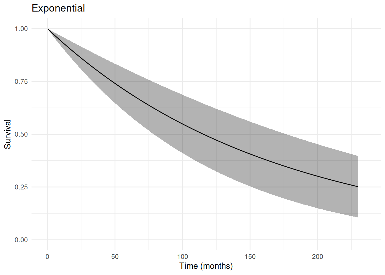

Weibull

The Weibull model is a two parameter model that is an extension of the exponential model. Here, the Weibull model is parameterized as h(t) = \lambda \gamma t^{\gamma - 1} where \gamma is the shape parameter. This parameter allows for the hazard to increase or decrease monotonically. The following code is used to fit a Weibull model.

# Define the estimating equation for the Weibull survival model
psi <- function(theta) {
  ee_survival_model(theta = theta,
                    time = d$times,
                    event = d$delta,
                    distribution = "weibull")
}

# Fit the M-estimator
estr <- m_estimate(stacked_equations = psi, init = c(0.01, 1.0))

# Display the results
results <- data.frame(
  Est = coef(estr),
  SE = sqrt(diag(vcov(estr))),
  LCL = confint(estr)[, 1],
  UCL = confint(estr)[, 2],
  row.names = c("Lambda", "Gamma")
)
round(results, 3)
#>          Est    SE   LCL   UCL
#> Lambda 0.010 0.005 0.000 0.019
#> Gamma  0.904 0.111 0.686 1.122

Here, \gamma is near 1, which suggests that the Weibull isn’t much better of a fit to the data.

As before, we can plot the survival function to get a better idea what these parameters mean.

# Compute survival predictions with confidence intervals
surv <- survival_predictions(
  times = times_to_predict,
  theta = coef(estr),
  covariance = vcov(estr),
  distribution = "weibull"
)

# Plot the survival function
ggplot(surv, aes(x = time, y = predicted)) +
  geom_ribbon(aes(ymin = lower, ymax = upper), fill = "black", alpha = 0.3) +
  geom_line() +
  coord_cartesian(xlim = c(0, 235), ylim = c(0, 1)) +
  labs(x = "Time (months)", y = "Survival", title = "Weibull")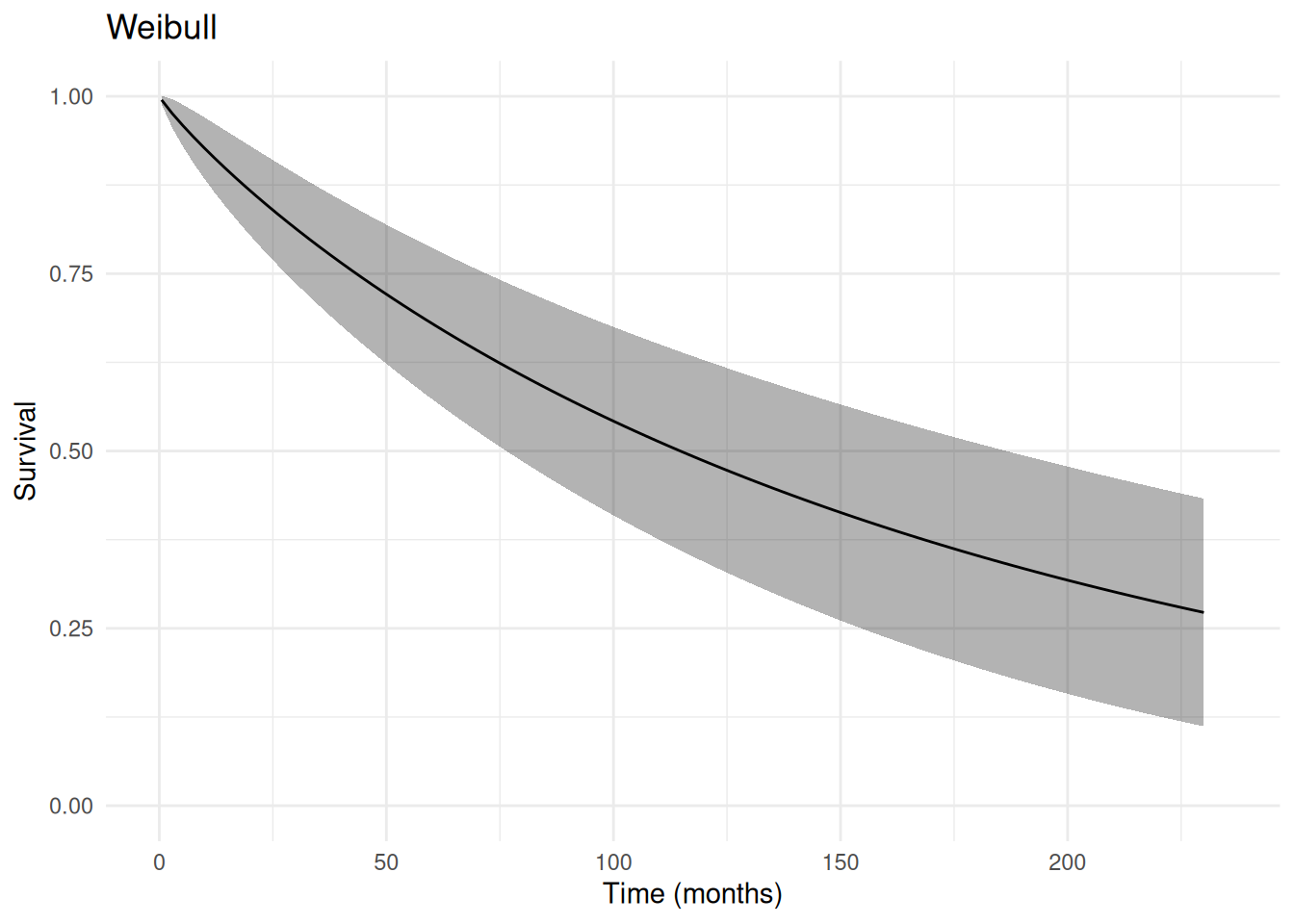

A disadvantage of the previous models is that they do not incorporate information on baseline covariates.

Chapter 6: Accelerated Failure Time and Other Parametric Models

Now we will switch focus to modeling survival by baseline covariates. The following is a line-diagram which represents the follow-up time for each individual (horizontal line), their event indicator (open circles are censoring, x’s are events), and the HPA stain status (shaded is negative).

In this case, we can see there seems to be some pattern in survival by HPA stain. However, there is censoring and our description here is pretty general. To help make our descriptions of survival differences more precise, we will use AFT models.

Here, we consider use of accelerated failure time (AFT) models with right censored data. These parametric models allow us to study how baseline variables are related to survival. AFT models are named because their scale parameters can be interpreted as how a baseline variable ‘accelerates’ the outcome. This acceleration is the ratio between the times when the survival are equal for a one unit change in the covariate. Alternatively, we can think about the parameters of this model as the ratio of mean survival times by covariate values.

The AFT model can be represented as a log-linear model: \log(T_i) = \beta_0 + \beta_1 X_i + \sigma \epsilon_i where different distributions for \epsilon provide different parametric AFT models. Here, \sigma is the shape parameter. It will be the parameter that varies in meaning between the different parametric distributions. The \beta’s are the scale factors which give us the acceleration factors, which can be interpreted as “the time to death given X=1 is accelerated by a factor of \exp(-\beta_1)”.

For further details on the structure and interpretation of AFT models, see the Collett book.

Exponential

To start, we consider the exponential AFT model. The exponential AFT model assumes a constant hazard, which is likely too simple for most settings. However, it can be useful to use as a starting point. The following is code to fit this AFT model using the ee_aft built-in estimating equation.

# Define the estimating equation for the exponential AFT model
psi <- function(theta) {
  ee_aft(theta = theta,
         X = as.matrix(d[, c("C", "stain")]),
         time = d$times,
         event = d$delta,
         distribution = "exponential")
}

# Fit the M-estimator
estr <- m_estimate(stacked_equations = psi, init = c(6.0, 0.0))

# Display the results
results <- data.frame(
  Est = coef(estr),
  SE = sqrt(diag(vcov(estr))),
  LCL = confint(estr)[, 1],
  UCL = confint(estr)[, 2],
  row.names = c("Intercept", "Stain")
)
round(results, 3)
#>              Est    SE    LCL   UCL
#> Intercept  5.800 0.431  4.956 6.645
#> Stain     -0.952 0.497 -1.926 0.023

Here, \exp(0.952) would be the acceleration factor due to a positive HPA stain (note the cancellation of the negative signs).

Another informative way to view these results is through a plot of the survival functions. The following code computes the survival function (at user-provided time points) for a specific covariate pattern. Here, we only consider HPA stain. The next block uses these predictions (and their confidence intervals) to plot the survival functions by HPA stain.

# Compute individual-level AFT predictions for each stain group
surv_neg <- aft_predictions_individual(
  X = matrix(c(1, 0), nrow = 1),
  times = times_to_predict,
  theta = coef(estr),
  distribution = "exponential"
)

surv_pos <- aft_predictions_individual(
  X = matrix(c(1, 1), nrow = 1),
  times = times_to_predict,
  theta = coef(estr),
  distribution = "exponential"
)

# Plot the survival functions by stain group
aft_surv <- data.frame(
  time = rep(times_to_predict, 2),
  survival = c(as.numeric(surv_neg), as.numeric(surv_pos)),
  stain = factor(
    rep(c("Negative", "Positive"), each = length(times_to_predict)),
    levels = c("Negative", "Positive")
  )
)

ggplot(aft_surv, aes(x = time, y = survival, color = stain)) +
  geom_line() +
  scale_color_manual(values = c(Negative = "blue", Positive = "red")) +
  coord_cartesian(xlim = c(0, 235), ylim = c(0, 1)) +
  labs(
    x = "Time (months)",
    y = "Survival",
    title = "Exponential AFT",
    color = NULL
  )

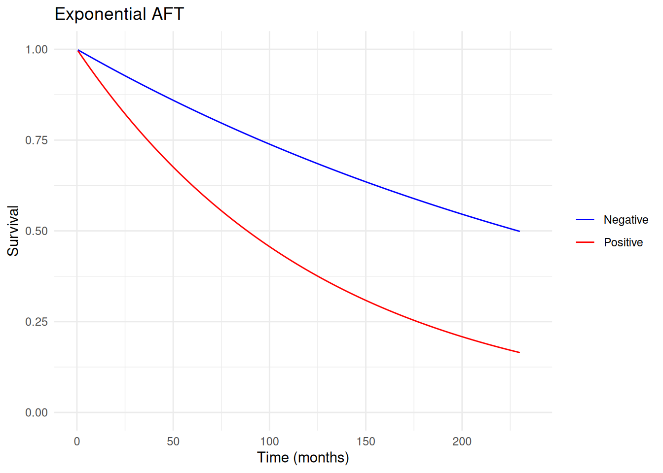
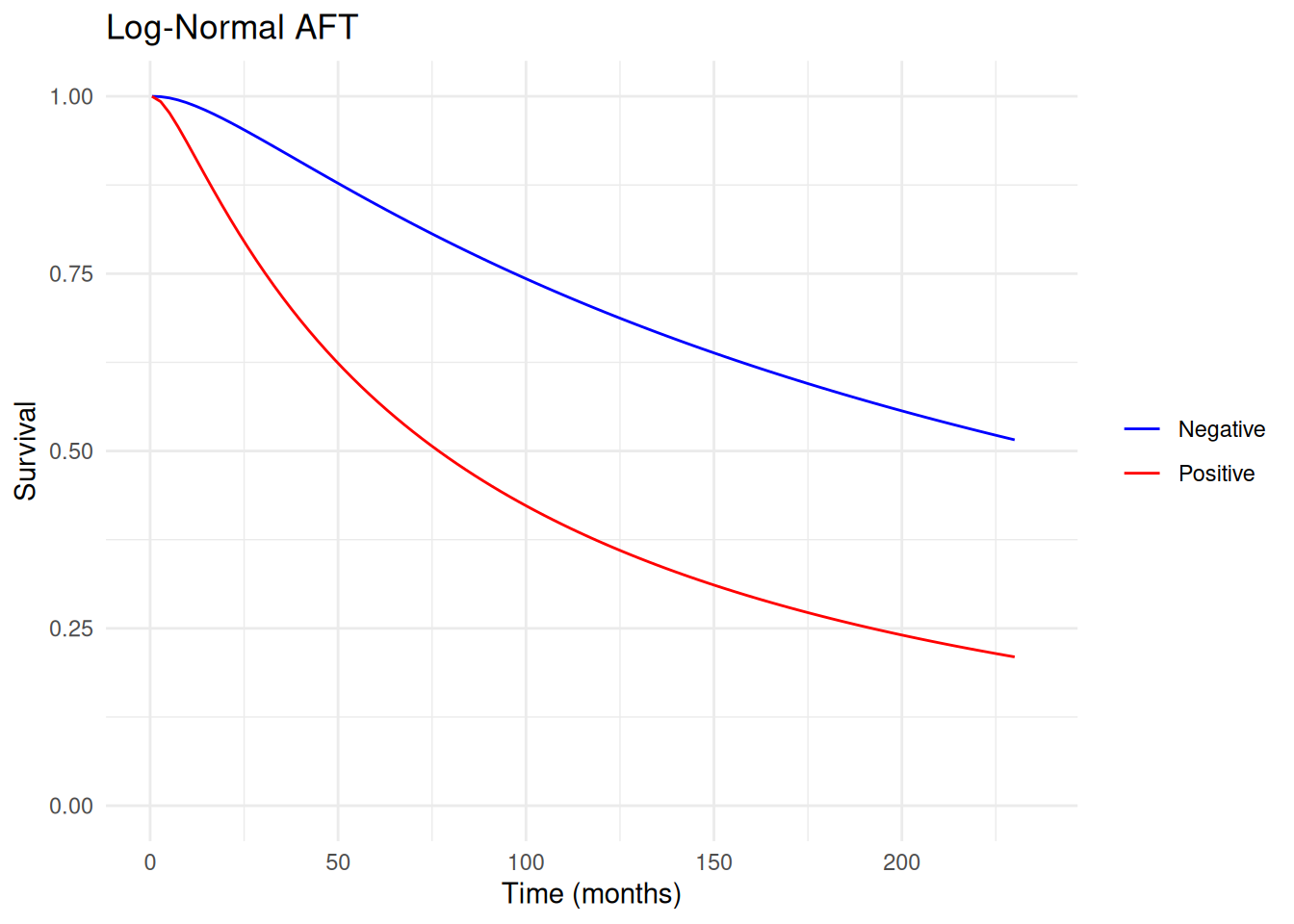
This plot summarizes how survival unfolds over time. These plots can be helpful with interpreting or presenting results beyond the table of estimated parameters given previously.

Weibull

The next model is the Weibull AFT model, which is a two-parameter generalization of the exponential model. In particular, it allows the hazard to vary in a specific monotonic way over time. To assess whether the exponential AFT model is reasonable, one can fit a Weibull model and assess whether the shape parameter (\sigma) is different from 1.

Below is how one can fit a Weibull AFT model with ee_aft.

# Define the estimating equation for the Weibull AFT model
psi <- function(theta) {
  ee_aft(theta = theta,
         X = as.matrix(d[, c("C", "stain")]),
         time = d$times,
         event = d$delta,
         distribution = "weibull")
}

# Fit the M-estimator
estr <- m_estimate(stacked_equations = psi, init = c(5.0, 0.0, 0.0))

# Display the results
results <- data.frame(
  Est = coef(estr),
  SE = sqrt(diag(vcov(estr))),
  LCL = confint(estr)[, 1],
  UCL = confint(estr)[, 2],
  row.names = c("Intercept", "Stain", "Shape")
)
round(results, 3)
#>              Est    SE    LCL   UCL
#> Intercept  5.854 0.483  4.909 6.800
#> Stain     -0.997 0.532 -2.039 0.046
#> Shape     -0.065 0.126 -0.311 0.182

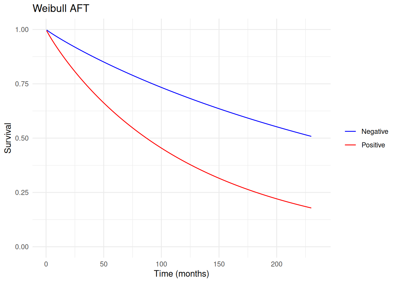
Note that the shape parameter here is the log-transformed version, so \exp(-0.065) is near one. This suggests that a Weibull AFT model provides a pretty similar fit to an exponential AFT model for this data. We can compare this to the results reported in Collett (pg 245). There we see that the intercept (\mu in Collett) and stain (\hat{\alpha} in Collett) match to the reported number of decimal places. Note that the \sigma in delicatessen is the inverse of the one reported in Collett.

Below is code to generate a plot of the survival functions. As the shape parameter is near one, this plot is expected to be similar to the exponential AFT model plot.

# Compute individual-level AFT predictions for each stain group
surv_neg <- aft_predictions_individual(
  X = matrix(c(1, 0), nrow = 1),
  times = times_to_predict,
  theta = coef(estr),
  distribution = "weibull"
)

surv_pos <- aft_predictions_individual(
  X = matrix(c(1, 1), nrow = 1),
  times = times_to_predict,
  theta = coef(estr),
  distribution = "weibull"
)

# Plot the survival functions by stain group
aft_surv <- data.frame(
  time = rep(times_to_predict, 2),
  survival = c(as.numeric(surv_neg), as.numeric(surv_pos)),
  stain = factor(
    rep(c("Negative", "Positive"), each = length(times_to_predict)),
    levels = c("Negative", "Positive")
  )
)

ggplot(aft_surv, aes(x = time, y = survival, color = stain)) +
  geom_line() +
  scale_color_manual(values = c(Negative = "blue", Positive = "red")) +
  coord_cartesian(xlim = c(0, 235), ylim = c(0, 1)) +
  labs(
    x = "Time (months)",
    y = "Survival",
    title = "Weibull AFT",
    color = NULL
  )

Other measures can also be plotted. Here, we plot the hazard functions shown in Figure 6.6 of Collett.

# Compute individual-level AFT hazard predictions for each stain group
haz_neg <- aft_predictions_individual(
  X = matrix(c(1, 0), nrow = 1),
  times = times_to_predict,
  theta = coef(estr),
  distribution = "weibull",
  measure = "hazard"
)

haz_pos <- aft_predictions_individual(
  X = matrix(c(1, 1), nrow = 1),
  times = times_to_predict,
  theta = coef(estr),
  distribution = "weibull",
  measure = "hazard"
)

# Plot the hazard functions by stain group
aft_haz <- data.frame(
  time = rep(times_to_predict, 2),
  hazard = c(as.numeric(haz_neg), as.numeric(haz_pos)),
  stain = factor(
    rep(c("Negative", "Positive"), each = length(times_to_predict)),
    levels = c("Negative", "Positive")
  )
)

ggplot(aft_haz, aes(x = time, y = hazard, color = stain)) +
  geom_line() +
  scale_color_manual(values = c(Negative = "blue", Positive = "red")) +
  coord_cartesian(xlim = c(-5, 235), ylim = c(0, 0.011)) +
  labs(
    x = "Time (months)",
    y = "Hazard",
    title = "Weibull AFT",
    color = NULL
  )

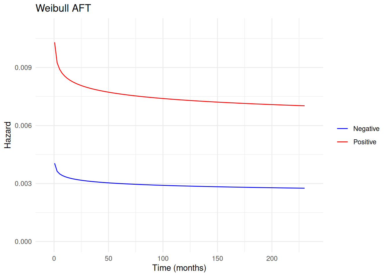
Note that the approximation near t=0 is less precise for the given spacing used. One could improve its appearance relative to the book by using a finer resolution.

Log-Normal

Another option is the log-normal AFT model. The following is how ee_aft can be used to fit the log-normal AFT model.

# Define the estimating equation for the log-normal AFT model
psi <- function(theta) {
  ee_aft(theta = theta,
         X = as.matrix(d[, c("C", "stain")]),
         time = d$times,
         event = d$delta,
         distribution = "log-normal")
}

# Fit the M-estimator
estr <- m_estimate(stacked_equations = psi, init = c(5.0, 0.0, 0.0))

# Display the results
results <- data.frame(
  Est = coef(estr),
  SE = sqrt(diag(vcov(estr))),
  LCL = confint(estr)[, 1],
  UCL = confint(estr)[, 2],
  row.names = c("Intercept", "Stain", "Shape")
)
round(results, 3)
#>              Est    SE    LCL    UCL
#> Intercept  5.492 0.450  4.609  6.374
#> Stain     -1.151 0.498 -2.127 -0.176
#> Shape     -0.307 0.134 -0.571 -0.043

# Compute individual-level AFT predictions for each stain group
surv_neg <- aft_predictions_individual(
  X = matrix(c(1, 0), nrow = 1),
  times = times_to_predict,
  theta = coef(estr),
  distribution = "log-normal"
)

surv_pos <- aft_predictions_individual(
  X = matrix(c(1, 1), nrow = 1),
  times = times_to_predict,
  theta = coef(estr),
  distribution = "log-normal"
)

# Plot the survival functions by stain group
aft_surv <- data.frame(
  time = rep(times_to_predict, 2),
  survival = c(as.numeric(surv_neg), as.numeric(surv_pos)),
  stain = factor(
    rep(c("Negative", "Positive"), each = length(times_to_predict)),
    levels = c("Negative", "Positive")
  )
)

ggplot(aft_surv, aes(x = time, y = survival, color = stain)) +
  geom_line() +
  scale_color_manual(values = c(Negative = "blue", Positive = "red")) +
  coord_cartesian(xlim = c(0, 235), ylim = c(0, 1)) +
  labs(
    x = "Time (months)",
    y = "Survival",
    title = "Log-Normal AFT",
    color = NULL
  )

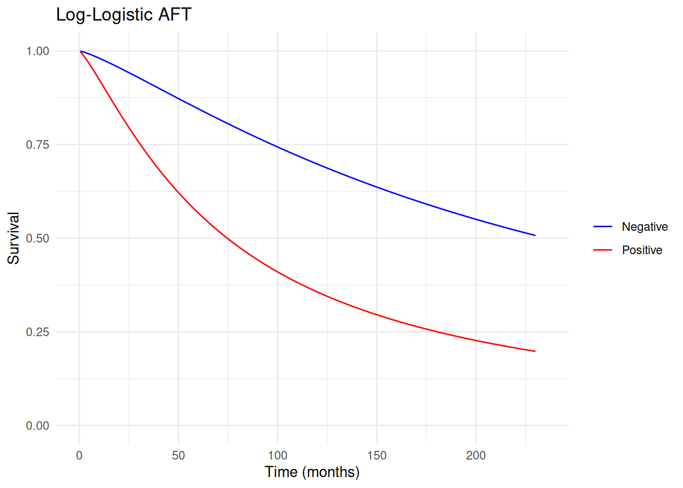
Log-Logistic

The final option available in delicatessen is the log-logistic AFT model. The following is how ee_aft can be used to fit this model.

# Define the estimating equation for the log-logistic AFT model
psi <- function(theta) {
  ee_aft(theta = theta,
         X = as.matrix(d[, c("C", "stain")]),
         time = d$times,
         event = d$delta,
         distribution = "log-logistic")
}

# Fit the M-estimator
estr <- m_estimate(stacked_equations = psi, init = c(5.0, 0.0, 0.0))

# Display the results
results <- data.frame(
  Est = coef(estr),
  SE = sqrt(diag(vcov(estr))),
  LCL = confint(estr)[, 1],
  UCL = confint(estr)[, 2],
  row.names = c("Intercept", "Stain", "Shape")
)
round(results, 3)
#>              Est    SE    LCL    UCL
#> Intercept  5.461 0.445  4.589  6.334
#> Stain     -1.149 0.505 -2.139 -0.159
#> Shape      0.217 0.145 -0.067  0.502

These parameter estimates are the same as those reported in Collett (except \sigma due to a differing parameterization).

# Compute individual-level AFT predictions for each stain group
surv_neg <- aft_predictions_individual(
  X = matrix(c(1, 0), nrow = 1),
  times = times_to_predict,
  theta = coef(estr),
  distribution = "log-logistic"
)

surv_pos <- aft_predictions_individual(
  X = matrix(c(1, 1), nrow = 1),
  times = times_to_predict,
  theta = coef(estr),
  distribution = "log-logistic"
)

# Plot the survival functions by stain group
aft_surv <- data.frame(
  time = rep(times_to_predict, 2),
  survival = c(as.numeric(surv_neg), as.numeric(surv_pos)),
  stain = factor(
    rep(c("Negative", "Positive"), each = length(times_to_predict)),
    levels = c("Negative", "Positive")
  )
)

ggplot(aft_surv, aes(x = time, y = survival, color = stain)) +
  geom_line() +
  scale_color_manual(values = c(Negative = "blue", Positive = "red")) +
  coord_cartesian(xlim = c(0, 235), ylim = c(0, 1)) +
  labs(
    x = "Time (months)",
    y = "Survival",
    title = "Log-Logistic AFT",
    color = NULL
  )

Again, we can also plot the hazard functions over time and compare them to the book (Figure 6.7).

# Compute individual-level AFT hazard predictions for each stain group
haz_neg <- aft_predictions_individual(
  X = matrix(c(1, 0), nrow = 1),
  times = times_to_predict,
  theta = coef(estr),
  distribution = "log-logistic",
  measure = "hazard"
)

haz_pos <- aft_predictions_individual(
  X = matrix(c(1, 1), nrow = 1),
  times = times_to_predict,
  theta = coef(estr),
  distribution = "log-logistic",
  measure = "hazard"
)

# Plot the hazard functions by stain group
aft_haz <- data.frame(
  time = rep(times_to_predict, 2),
  hazard = c(as.numeric(haz_neg), as.numeric(haz_pos)),
  stain = factor(
    rep(c("Negative", "Positive"), each = length(times_to_predict)),
    levels = c("Negative", "Positive")
  )
)

ggplot(aft_haz, aes(x = time, y = hazard, color = stain)) +
  geom_line() +
  scale_color_manual(values = c(Negative = "blue", Positive = "red")) +
  coord_cartesian(xlim = c(-5, 235), ylim = c(0, 0.011)) +
  labs(
    x = "Time (months)",
    y = "Hazard",
    title = "Log-Logistic AFT",
    color = NULL
  )

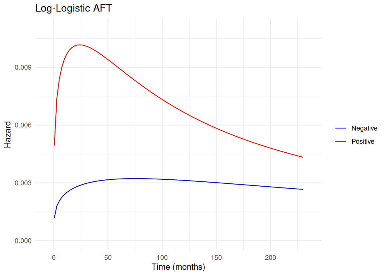
Consistent with the other results, the log-logistic AFT model does not differ substantially from the other AFT models.

Here, we applied some of the parametric survival models described at length in Collett using the M-estimation framework. As these models are all finite dimension parameter vectors, standard M-estimation theory straightforwardly applies. A benefit in this context is the ease that variance estimation can be accomplished to create plots with point-wise confidence intervals.

References

Collett, D. (2015). Survival analysis. In Modelling survival data in medical research. 3rd Ed. Chapman and Hall/CRC. pg 6-7

Collett, D. (2015). Accelerated failure time and other parametric models. In Modelling survival data in medical research. 3rd Ed. Chapman and Hall/CRC. pg 221-274